qp Demo
Note: This is a legacy notebook created for qp version < 1. Some of this notebook may no longer be accurate for qp version >= 1. It is kept availablle for reference.
Alex Malz, Phil Marshall, Eric Charles
In this notebook we use the qp module to approximate some simple, standard, 1D PDFs using sets of quantiles, samples, and histograms, and assess their relative accuracy.
We also show how such analyses can be extended to use “composite” PDFs made up of mixtures of standard distributions.
import numpy as np
import os
import scipy.stats as sps

import matplotlib
matplotlib.use('Agg')
import matplotlib.pyplot as plt
%matplotlib inline
Requirements
To run qp, you will need to first install the module by following the instructions here.
import qp
Background: the scipy.stats module
The scipy.stats module is the standard for manipulating distribtions so is a natural place to start for implementing 1D PDF parameterizations.
It allows you do define a wide variety of distibutions and uses numpy array broadcasting for efficiency.
Gaussian (Normal) example
Here are some examples of things you can do with the scipy.stats module, using a Gaussian or Normal distribution.
loc and scale are the means and standard deviations of the underlying Gaussians.
Note the distinction between passing arguments to norm and passing arguments to pdf to access multiple distributions and their PDF values at multiple points.
# evaluate a single distribution's PDF at one value
print("PDF at one point for one distribution:",
      sps.norm(loc=0, scale=1).pdf(0.5))

# evaluate a single distribution's PDF at multiple value
print("PDF at three points for one distribution:",
      sps.norm(loc=0, scale=1).pdf([0.5, 1., 1.5]))

# evalute three distributions' PDFs at one shared value
print("PDF at one point for three distributions:",
      sps.norm(loc=[0., 1., 2.], scale=1).pdf(0.5))

# evalute three distributions' PDFs each at one different value
print("PDF at one different point for three distributions:",
      sps.norm(loc=[0., 1., 2.], scale=1).pdf([0.5, 1., 1.5]))

# evalute three distributions' PDFs each at four different values
# (note the change in shape of the argument)
print("PDF at four different points for three distributions:\n",
      sps.norm(loc=[0., 1., 2.], scale=1).pdf([[0.5],[1.],[1.5],[2]]))

# evalute three distributions' PDFs at each of four different values
# (note the change in shape of the argument)
print("PDF at four different points for three distributions: broadcast reversed\n",
      sps.norm(loc=[[0.], [1.], [2.]], scale=1).pdf([0.5,1.,1.5,2]))
PDF at one point for one distribution: 0.3520653267642995
PDF at three points for one distribution: [0.35206533 0.24197072 0.1295176 ]
PDF at one point for three distributions: [0.35206533 0.35206533 0.1295176 ]
PDF at one different point for three distributions: [0.35206533 0.39894228 0.35206533]
PDF at four different points for three distributions:
 [[0.35206533 0.35206533 0.1295176 ]
 [0.24197072 0.39894228 0.24197072]
 [0.1295176  0.35206533 0.35206533]
 [0.05399097 0.24197072 0.39894228]]
PDF at four different points for three distributions: broadcast reversed
 [[0.35206533 0.24197072 0.1295176  0.05399097]
 [0.35206533 0.39894228 0.35206533 0.24197072]
 [0.1295176  0.24197072 0.35206533 0.39894228]]
The scipy.stats classes
In the scipy.stats module, all of the distributions are sub-classes of scipy.stats.rv_continuous.
You make an object of a particular sub-type, and then ‘freeze’ it by passing it shape parameters.
print("This is the generic normal distribution class: ",
      sps._continuous_distns.norm_gen)

ng = sps._continuous_distns.norm_gen()
print("This is an instance of the generic normal distribution class",
      ng)

norm_sp = ng(loc=0, scale=1)
print("This is a frozen normal distribution, with specific paramters",
      norm_sp, norm_sp.kwds)
print("The frozen object know what generic distribution it comes from",
      norm_sp.dist)
This is the generic normal distribution class:  <class 'scipy.stats._continuous_distns.norm_gen'>
This is an instance of the generic normal distribution class <scipy.stats._continuous_distns.norm_gen object at 0x73d5153b3eb0>
This is a frozen normal distribution, with specific paramters <scipy.stats._distn_infrastructure.rv_continuous_frozen object at 0x73d5153b1d80> {'loc': 0, 'scale': 1}
The frozen object know what generic distribution it comes from <scipy.stats._continuous_distns.norm_gen object at 0x73d5153b36d0>
Properties of distributions
scipy.stats lets you evaluate multiple properties of distributions. These include:
pdf: Probability Density Function
cdf: Cumulative Distribution Function
ppf: Percent Point Function (Inverse of CDF)
sf: Survival Function (1-CDF)
isf: Inverse Survival Function (Inverse of SF)
rvs: Random Variates (i.e., sampled values)
stats: Return mean, variance, optionally: (Fisher’s) skew, or (Fisher’s) kurtosis
moment: non-central moments of the distribution
print("PDF = ", norm_sp.pdf(0.5))
print("CDF = ", norm_sp.cdf(0.5))
print("PPF = ", norm_sp.ppf(0.6))
print("SF  = ", norm_sp.sf(0.6))
print("ISF = ", norm_sp.isf(0.5))
print("RVS = ", norm_sp.rvs())
print("stats = ", norm_sp.stats())
print("M2  = ", norm_sp.moment(2))
PDF =  0.3520653267642995
CDF =  0.6914624612740131
PPF =  0.2533471031357997
SF  =  0.2742531177500736
ISF =  0.0
RVS =  -1.019837753306423
stats =  (np.float64(0.0), np.float64(1.0))
M2  =  1.0
qp parameterizations and visualization functionality
The next part of this notebook shows how we can extend the functionality of scipy.stats to implement distributions that are based on parameterizations of 1D PDFs, like histograms, interpolations, splines, or mixture models.
Parameterizations from scipy.stats
qp automatically generates classes for all of the scipy.stats.rv_continuous distributions, providing feed-through access to all scipy.stats.rv_continuous objects but adds on additional attributes and methods specific to parameterization conversions.
qp.stats.keys()
odict_keys(['alpha', 'anglit', 'arcsine', 'argus', 'beta', 'betaprime', 'bradford', 'burr', 'burr12', 'cauchy', 'chi', 'chi2', 'cosine', 'crystalball', 'dgamma', 'dpareto_lognorm', 'dweibull', 'erlang', 'expon', 'exponnorm', 'exponpow', 'exponweib', 'f', 'fatiguelife', 'fisk', 'foldcauchy', 'foldnorm', 'gamma', 'gausshyper', 'genexpon', 'genextreme', 'gengamma', 'genhalflogistic', 'genhyperbolic', 'geninvgauss', 'genlogistic', 'gennorm', 'genpareto', 'gibrat', 'gompertz', 'gumbel_l', 'gumbel_r', 'halfcauchy', 'halfgennorm', 'halflogistic', 'halfnorm', 'hypsecant', 'invgamma', 'invgauss', 'invweibull', 'irwinhall', 'jf_skew_t', 'johnsonsb', 'johnsonsu', 'kappa3', 'kappa4', 'ksone', 'kstwo', 'kstwobign', 'landau', 'laplace', 'laplace_asymmetric', 'levy', 'levy_l', 'levy_stable', 'loggamma', 'logistic', 'loglaplace', 'lognorm', 'loguniform', 'lomax', 'maxwell', 'mielke', 'moyal', 'nakagami', 'ncf', 'nct', 'ncx2', 'norm', 'norminvgauss', 'pareto', 'pearson3', 'powerlaw', 'powerlognorm', 'powernorm', 'rayleigh', 'rdist', 'recipinvgauss', 'reciprocal', 'rel_breitwigner', 'rice', 'semicircular', 'skewcauchy', 'skewnorm', 'studentized_range', 't', 'trapezoid', 'trapz', 'triang', 'truncexpon', 'truncnorm', 'truncpareto', 'truncweibull_min', 'tukeylambda', 'uniform', 'vonmises', 'vonmises_line', 'wald', 'weibull_max', 'weibull_min', 'wrapcauchy', 'spline', 'hist', 'interp', 'interp_irregular', 'quant', 'mixmod', 'sparse', 'packed_interp'])
help(qp.stats.lognorm_gen)
Help on class lognorm in module qp.core.factory:
class lognorm(qp.parameterizations.base.Pdf_gen_wrap, scipy.stats._continuous_distns.lognorm_gen)
| lognorm(*args, **kwargs)
|
| A lognormal continuous random variable.
|
| %(before_notes)s
|
| Notes
| -----
| The probability density function for `lognorm` is:
|
| .. math::
|
| f(x, s) = \frac{1}{s x \sqrt{2\pi}}
| \exp\left(-\frac{\log^2(x)}{2s^2}\right)
|
| for :math:`x > 0`, :math:`s > 0`.
|
| `lognorm` takes ``s`` as a shape parameter for :math:`s`.
|
| %(after_notes)s
|
| Suppose a normally distributed random variable ``X`` has mean ``mu`` and
| standard deviation ``sigma``. Then ``Y = exp(X)`` is lognormally
| distributed with ``s = sigma`` and ``scale = exp(mu)``.
|
| %(example)s
|
| The logarithm of a log-normally distributed random variable is
| normally distributed:
|
| >>> import numpy as np
| >>> import matplotlib.pyplot as plt
| >>> from scipy import stats
| >>> fig, ax = plt.subplots(1, 1)
| >>> mu, sigma = 2, 0.5
| >>> X = stats.norm(loc=mu, scale=sigma)
| >>> Y = stats.lognorm(s=sigma, scale=np.exp(mu))
| >>> x = np.linspace(*X.interval(0.999))
| >>> y = Y.rvs(size=10000)
| >>> ax.plot(x, X.pdf(x), label='X (pdf)')
| >>> ax.hist(np.log(y), density=True, bins=x, label='log(Y) (histogram)')
| >>> ax.legend()
| >>> plt.show()
|
| Method resolution order:
| lognorm
| qp.parameterizations.base.Pdf_gen_wrap
| qp.parameterizations.base.Pdf_gen
| scipy.stats._continuous_distns.lognorm_gen
| scipy.stats._distn_infrastructure.rv_continuous
| scipy.stats._distn_infrastructure.rv_generic
| builtins.object
|
| Methods defined here:
|
| create_ensemble(data: 'Mapping', ancil: 'Optional[Mapping]' = None) -> 'Ensemble'
| Creates an Ensemble of distribution(s) in the given parameterization.
|
| Input data format:
| data = {'arg1': values, 'arg2': values ...} where 'arg1', 'arg2'... are the arguments for the parameterization.
| The length of the values should be the number of distributions being created in the Ensemble, with a minimum value of 1.
|
|
| Parameters
| ----------
| data : Mapping
| The dictionary of data for the distributions.
| ancil : Optional[Mapping], optional
| A dictionary of metadata for the distributions, where any arrays have the same length as the number of distributions, by default None
|
| Returns
| -------
| Ensemble
| An Ensemble object containing all of the given distributions.
|
| Examples
| --------
|
| To create an Ensemble with two Gaussian distributions and their associated ids:
|
| >>> import qp
| >>> data = {'loc': np.array([[0.45],[0.55]]) , 'scale': np.array([[0.2],[0.15]])}
| >>> ancil = {'ids': [20,25]}
| >>> ens = qp.stats.norm.create_ensemble(data,ancil)
| >>> ens.metadata
| {'pdf_name': array([b'norm'], dtype='|S4'), 'pdf_version': array([0])}
|
| freeze = _my_freeze(self, *args, **kwds)
|
| ----------------------------------------------------------------------
| Data and other attributes defined here:
|
| name = 'lognorm'
|
| version = 0
|
| ----------------------------------------------------------------------
| Methods inherited from qp.parameterizations.base.Pdf_gen_wrap:
|
| __init__(self, *args, **kwargs)
| C'tor
|
| ----------------------------------------------------------------------
| Class methods inherited from qp.parameterizations.base.Pdf_gen_wrap:
|
| add_mappings() from builtins.type
| Add this classes mappings to the conversion dictionary
|
| create(**kwds) from builtins.type
| Create and return a `scipy.stats.rv_frozen` object using the
| keyword arguments provided
|
| create_gen(**kwds) from builtins.type
| Create and return a `scipy.stats.rv_continuous` object using the
| keyword arguments provided
|
| get_allocation_kwds(npdf, **kwargs) from builtins.type
| Return kwds necessary to create 'empty' hdf5 file with npdf entries
| for iterative writeout
|
| ----------------------------------------------------------------------
| Class methods inherited from qp.parameterizations.base.Pdf_gen:
|
| add_method_dicts() from builtins.type
| Add empty method dicts
|
| creation_method(method=None) from builtins.type
| Return the method used to create a PDF of this type
|
| extraction_method(method=None) from builtins.type
| Return the method used to extract data to create a PDF of this type
|
| plot(pdf, **kwargs) from builtins.type
| Plot the pdf as a curve
|
| plot_native(pdf, **kwargs) from builtins.type
| Plot the PDF in a way that is particular to this type of distribution
|
| This defaults to plotting it as a curve, but this can be overwritten
|
| print_method_maps(stream=<ipykernel.iostream.OutStream object at 0x73d5533de3b0>) from builtins.type
| Print the maps showing the methods
|
| reader_method(version=None) from builtins.type
| Return the method used to convert data read from a file PDF of this type
|
| ----------------------------------------------------------------------
| Readonly properties inherited from qp.parameterizations.base.Pdf_gen:
|
| metadata
| Return the metadata for this set of PDFs
|
| objdata
| Return the object data for this set of PDFs
|
| ----------------------------------------------------------------------
| Data descriptors inherited from qp.parameterizations.base.Pdf_gen:
|
| __dict__
| dictionary for instance variables (if defined)
|
| __weakref__
| list of weak references to the object (if defined)
|
| ----------------------------------------------------------------------
| Methods inherited from scipy.stats._continuous_distns.lognorm_gen:
|
| fit(self, data, *args, **kwds)
| Return estimates of shape (if applicable), location, and scale
| parameters from data. The default estimation method is Maximum
| Likelihood Estimation (MLE), but Method of Moments (MM)
| is also available.
|
| Starting estimates for the fit are given by input arguments;
| for any arguments not provided with starting estimates,
| ``self._fitstart(data)`` is called to generate such.
|
| One can hold some parameters fixed to specific values by passing in
| keyword arguments ``f0``, ``f1``, ..., ``fn`` (for shape parameters)
| and ``floc`` and ``fscale`` (for location and scale parameters,
| respectively).
|
| Parameters
| ----------
| data : array_like or `CensoredData` instance
| Data to use in estimating the distribution parameters.
| arg1, arg2, arg3,... : floats, optional
| Starting value(s) for any shape-characterizing arguments (those not
| provided will be determined by a call to ``_fitstart(data)``).
| No default value.
| **kwds : floats, optional
| - `loc`: initial guess of the distribution's location parameter.
| - `scale`: initial guess of the distribution's scale parameter.
|
| Special keyword arguments are recognized as holding certain
| parameters fixed:
|
| - f0...fn : hold respective shape parameters fixed.
| Alternatively, shape parameters to fix can be specified by name.
| For example, if ``self.shapes == "a, b"``, ``fa`` and ``fix_a``
| are equivalent to ``f0``, and ``fb`` and ``fix_b`` are
| equivalent to ``f1``.
|
| - floc : hold location parameter fixed to specified value.
|
| - fscale : hold scale parameter fixed to specified value.
|
| - optimizer : The optimizer to use. The optimizer must take
| ``func`` and starting position as the first two arguments,
| plus ``args`` (for extra arguments to pass to the
| function to be optimized) and ``disp``.
| The ``fit`` method calls the optimizer with ``disp=0`` to suppress output.
| The optimizer must return the estimated parameters.
|
| - method : The method to use. The default is "MLE" (Maximum
| Likelihood Estimate); "MM" (Method of Moments)
| is also available.
|
| Raises
| ------
| TypeError, ValueError
| If an input is invalid
| `~scipy.stats.FitError`
| If fitting fails or the fit produced would be invalid
|
| Returns
| -------
| parameter_tuple : tuple of floats
| Estimates for any shape parameters (if applicable), followed by
| those for location and scale. For most random variables, shape
| statistics will be returned, but there are exceptions (e.g.
| ``norm``).
|
| Notes
| -----
| With ``method="MLE"`` (default), the fit is computed by minimizing
| the negative log-likelihood function. A large, finite penalty
| (rather than infinite negative log-likelihood) is applied for
| observations beyond the support of the distribution.
|
| With ``method="MM"``, the fit is computed by minimizing the L2 norm
| of the relative errors between the first *k* raw (about zero) data
| moments and the corresponding distribution moments, where *k* is the
| number of non-fixed parameters.
| More precisely, the objective function is::
|
| (((data_moments - dist_moments)
| / np.maximum(np.abs(data_moments), 1e-8))**2).sum()
|
| where the constant ``1e-8`` avoids division by zero in case of
| vanishing data moments. Typically, this error norm can be reduced to
| zero.
| Note that the standard method of moments can produce parameters for
| which some data are outside the support of the fitted distribution;
| this implementation does nothing to prevent this.
|
| For either method,
| the returned answer is not guaranteed to be globally optimal; it
| may only be locally optimal, or the optimization may fail altogether.
| If the data contain any of ``np.nan``, ``np.inf``, or ``-np.inf``,
| the `fit` method will raise a ``RuntimeError``.
|
| When passing a ``CensoredData`` instance to ``data``, the log-likelihood
| function is defined as:
|
| .. math::
|
| l(\pmb{\theta}; k) & = \sum
| \log(f(k_u; \pmb{\theta}))
| + \sum
| \log(F(k_l; \pmb{\theta})) \\
| & + \sum
| \log(1 - F(k_r; \pmb{\theta})) \\
| & + \sum
| \log(F(k_{\text{high}, i}; \pmb{\theta})
| - F(k_{\text{low}, i}; \pmb{\theta}))
|
| where :math:`f` and :math:`F` are the pdf and cdf, respectively, of the
| function being fitted, :math:`\pmb{\theta}` is the parameter vector,
| :math:`u` are the indices of uncensored observations,
| :math:`l` are the indices of left-censored observations,
| :math:`r` are the indices of right-censored observations,
| subscripts "low"/"high" denote endpoints of interval-censored observations, and
| :math:`i` are the indices of interval-censored observations.
|
| When `method='MLE'` and
| the location parameter is fixed by using the `floc` argument,
| this function uses explicit formulas for the maximum likelihood
| estimation of the log-normal shape and scale parameters, so the
| `optimizer`, `loc` and `scale` keyword arguments are ignored.
| If the location is free, a likelihood maximum is found by
| setting its partial derivative wrt to location to 0, and
| solving by substituting the analytical expressions of shape
| and scale (or provided parameters).
| See, e.g., equation 3.1 in
| A. Clifford Cohen & Betty Jones Whitten (1980)
| Estimation in the Three-Parameter Lognormal Distribution,
| Journal of the American Statistical Association, 75:370, 399-404
| https://doi.org/10.2307/2287466
|
|
| Examples
| --------
|
| Generate some data to fit: draw random variates from the `beta`
| distribution
|
| >>> import numpy as np
| >>> from scipy.stats import beta
| >>> a, b = 1., 2.
| >>> rng = np.random.default_rng(172786373191770012695001057628748821561)
| >>> x = beta.rvs(a, b, size=1000, random_state=rng)
|
| Now we can fit all four parameters (``a``, ``b``, ``loc`` and
| ``scale``):
|
| >>> a1, b1, loc1, scale1 = beta.fit(x)
| >>> a1, b1, loc1, scale1
| (1.0198945204435628, 1.9484708982737828, 4.372241314917588e-05, 0.9979078845964814)
|
| The fit can be done also using a custom optimizer:
|
| >>> from scipy.optimize import minimize
| >>> def custom_optimizer(func, x0, args=(), disp=0):
| ... res = minimize(func, x0, args, method="slsqp", options={"disp": disp})
| ... if res.success:
| ... return res.x
| ... raise RuntimeError('optimization routine failed')
| >>> a1, b1, loc1, scale1 = beta.fit(x, method="MLE", optimizer=custom_optimizer)
| >>> a1, b1, loc1, scale1
| (1.0198821087258905, 1.948484145914738, 4.3705304486881485e-05, 0.9979104663953395)
|
| We can also use some prior knowledge about the dataset: let's keep
| ``loc`` and ``scale`` fixed:
|
| >>> a1, b1, loc1, scale1 = beta.fit(x, floc=0, fscale=1)
| >>> loc1, scale1
| (0, 1)
|
| We can also keep shape parameters fixed by using ``f``-keywords. To
| keep the zero-th shape parameter ``a`` equal 1, use ``f0=1`` or,
| equivalently, ``fa=1``:
|
| >>> a1, b1, loc1, scale1 = beta.fit(x, fa=1, floc=0, fscale=1)
| >>> a1
| 1
|
| Not all distributions return estimates for the shape parameters.
| ``norm`` for example just returns estimates for location and scale:
|
| >>> from scipy.stats import norm
| >>> x = norm.rvs(a, b, size=1000, random_state=123)
| >>> loc1, scale1 = norm.fit(x)
| >>> loc1, scale1
| (0.92087172783841631, 2.0015750750324668)
|
| ----------------------------------------------------------------------
| Methods inherited from scipy.stats._distn_infrastructure.rv_continuous:
|
| __getstate__(self)
|
| cdf(self, x, *args, **kwds)
| Cumulative distribution function of the given RV.
|
| Parameters
| ----------
| x : array_like
| quantiles
| arg1, arg2, arg3,... : array_like
| The shape parameter(s) for the distribution (see docstring of the
| instance object for more information)
| loc : array_like, optional
| location parameter (default=0)
| scale : array_like, optional
| scale parameter (default=1)
|
| Returns
| -------
| cdf : ndarray
| Cumulative distribution function evaluated at `x`
|
| expect(self, func=None, args=(), loc=0, scale=1, lb=None, ub=None, conditional=False, **kwds)
| Calculate expected value of a function with respect to the
| distribution by numerical integration.
|
| The expected value of a function ``f(x)`` with respect to a
| distribution ``dist`` is defined as::
|
| ub
| E[f(x)] = Integral(f(x) * dist.pdf(x)),
| lb
|
| where ``ub`` and ``lb`` are arguments and ``x`` has the ``dist.pdf(x)``
| distribution. If the bounds ``lb`` and ``ub`` correspond to the
| support of the distribution, e.g. ``[-inf, inf]`` in the default
| case, then the integral is the unrestricted expectation of ``f(x)``.
| Also, the function ``f(x)`` may be defined such that ``f(x)`` is ``0``
| outside a finite interval in which case the expectation is
| calculated within the finite range ``[lb, ub]``.
|
| Parameters
| ----------
| func : callable, optional
| Function for which integral is calculated. Takes only one argument.
| The default is the identity mapping f(x) = x.
| args : tuple, optional
| Shape parameters of the distribution.
| loc : float, optional
| Location parameter (default=0).
| scale : float, optional
| Scale parameter (default=1).
| lb, ub : scalar, optional
| Lower and upper bound for integration. Default is set to the
| support of the distribution.
| conditional : bool, optional
| If True, the integral is corrected by the conditional probability
| of the integration interval. The return value is the expectation
| of the function, conditional on being in the given interval.
| Default is False.
|
| Additional keyword arguments are passed to the integration routine.
|
| Returns
| -------
| expect : float
| The calculated expected value.
|
| Notes
| -----
| The integration behavior of this function is inherited from
| `scipy.integrate.quad`. Neither this function nor
| `scipy.integrate.quad` can verify whether the integral exists or is
| finite. For example ``cauchy(0).mean()`` returns ``np.nan`` and
| ``cauchy(0).expect()`` returns ``0.0``.
|
| Likewise, the accuracy of results is not verified by the function.
| `scipy.integrate.quad` is typically reliable for integrals that are
| numerically favorable, but it is not guaranteed to converge
| to a correct value for all possible intervals and integrands. This
| function is provided for convenience; for critical applications,
| check results against other integration methods.
|
| The function is not vectorized.
|
| Examples
| --------
|
| To understand the effect of the bounds of integration consider
|
| >>> from scipy.stats import expon
| >>> expon(1).expect(lambda x: 1, lb=0.0, ub=2.0)
| 0.6321205588285578
|
| This is close to
|
| >>> expon(1).cdf(2.0) - expon(1).cdf(0.0)
| 0.6321205588285577
|
| If ``conditional=True``
|
| >>> expon(1).expect(lambda x: 1, lb=0.0, ub=2.0, conditional=True)
| 1.0000000000000002
|
| The slight deviation from 1 is due to numerical integration.
|
| The integrand can be treated as a complex-valued function
| by passing ``complex_func=True`` to `scipy.integrate.quad` .
|
| >>> import numpy as np
| >>> from scipy.stats import vonmises
| >>> res = vonmises(loc=2, kappa=1).expect(lambda x: np.exp(1j*x),
| ... complex_func=True)
| >>> res
| (-0.18576377217422957+0.40590124735052263j)
|
| >>> np.angle(res) # location of the (circular) distribution
| 2.0
|
| fit_loc_scale(self, data, *args)
| Estimate loc and scale parameters from data using 1st and 2nd moments.
|
| Parameters
| ----------
| data : array_like
| Data to fit.
| arg1, arg2, arg3,... : array_like
| The shape parameter(s) for the distribution (see docstring of the
| instance object for more information).
|
| Returns
| -------
| Lhat : float
| Estimated location parameter for the data.
| Shat : float
| Estimated scale parameter for the data.
|
| isf(self, q, *args, **kwds)
| Inverse survival function (inverse of `sf`) at q of the given RV.
|
| Parameters
| ----------
| q : array_like
| upper tail probability
| arg1, arg2, arg3,... : array_like
| The shape parameter(s) for the distribution (see docstring of the
| instance object for more information)
| loc : array_like, optional
| location parameter (default=0)
| scale : array_like, optional
| scale parameter (default=1)
|
| Returns
| -------
| x : ndarray or scalar
| Quantile corresponding to the upper tail probability q.
|
| logcdf(self, x, *args, **kwds)
| Log of the cumulative distribution function at x of the given RV.
|
| Parameters
| ----------
| x : array_like
| quantiles
| arg1, arg2, arg3,... : array_like
| The shape parameter(s) for the distribution (see docstring of the
| instance object for more information)
| loc : array_like, optional
| location parameter (default=0)
| scale : array_like, optional
| scale parameter (default=1)
|
| Returns
| -------
| logcdf : array_like
| Log of the cumulative distribution function evaluated at x
|
| logpdf(self, x, *args, **kwds)
| Log of the probability density function at x of the given RV.
|
| This uses a more numerically accurate calculation if available.
|
| Parameters
| ----------
| x : array_like
| quantiles
| arg1, arg2, arg3,... : array_like
| The shape parameter(s) for the distribution (see docstring of the
| instance object for more information)
| loc : array_like, optional
| location parameter (default=0)
| scale : array_like, optional
| scale parameter (default=1)
|
| Returns
| -------
| logpdf : array_like
| Log of the probability density function evaluated at x
|
| logsf(self, x, *args, **kwds)
| Log of the survival function of the given RV.
|
| Returns the log of the "survival function," defined as (1 - `cdf`),
| evaluated at `x`.
|
| Parameters
| ----------
| x : array_like
| quantiles
| arg1, arg2, arg3,... : array_like
| The shape parameter(s) for the distribution (see docstring of the
| instance object for more information)
| loc : array_like, optional
| location parameter (default=0)
| scale : array_like, optional
| scale parameter (default=1)
|
| Returns
| -------
| logsf : ndarray
| Log of the survival function evaluated at `x`.
|
| pdf(self, x, *args, **kwds)
| Probability density function at x of the given RV.
|
| Parameters
| ----------
| x : array_like
| quantiles
| arg1, arg2, arg3,... : array_like
| The shape parameter(s) for the distribution (see docstring of the
| instance object for more information)
| loc : array_like, optional
| location parameter (default=0)
| scale : array_like, optional
| scale parameter (default=1)
|
| Returns
| -------
| pdf : ndarray
| Probability density function evaluated at x
|
| ppf(self, q, *args, **kwds)
| Percent point function (inverse of `cdf`) at q of the given RV.
|
| Parameters
| ----------
| q : array_like
| lower tail probability
| arg1, arg2, arg3,... : array_like
| The shape parameter(s) for the distribution (see docstring of the
| instance object for more information)
| loc : array_like, optional
| location parameter (default=0)
| scale : array_like, optional
| scale parameter (default=1)
|
| Returns
| -------
| x : array_like
| quantile corresponding to the lower tail probability q.
|
| sf(self, x, *args, **kwds)
| Survival function (1 - `cdf`) at x of the given RV.
|
| Parameters
| ----------
| x : array_like
| quantiles
| arg1, arg2, arg3,... : array_like
| The shape parameter(s) for the distribution (see docstring of the
| instance object for more information)
| loc : array_like, optional
| location parameter (default=0)
| scale : array_like, optional
| scale parameter (default=1)
|
| Returns
| -------
| sf : array_like
| Survival function evaluated at x
|
| ----------------------------------------------------------------------
| Methods inherited from scipy.stats._distn_infrastructure.rv_generic:
|
| __call__(self, *args, **kwds)
| Freeze the distribution for the given arguments.
|
| Parameters
| ----------
| arg1, arg2, arg3,... : array_like
| The shape parameter(s) for the distribution. Should include all
| the non-optional arguments, may include ``loc`` and ``scale``.
|
| Returns
| -------
| rv_frozen : rv_frozen instance
| The frozen distribution.
|
| __setstate__(self, state)
|
| entropy(self, *args, **kwds)
| Differential entropy of the RV.
|
| Parameters
| ----------
| arg1, arg2, arg3,... : array_like
| The shape parameter(s) for the distribution (see docstring of the
| instance object for more information).
| loc : array_like, optional
| Location parameter (default=0).
| scale : array_like, optional (continuous distributions only).
| Scale parameter (default=1).
|
| Notes
| -----
| Entropy is defined base `e`:
|
| >>> import numpy as np
| >>> from scipy.stats._distn_infrastructure import rv_discrete
| >>> drv = rv_discrete(values=((0, 1), (0.5, 0.5)))
| >>> np.allclose(drv.entropy(), np.log(2.0))
| True
|
| interval(self, confidence, *args, **kwds)
| Confidence interval with equal areas around the median.
|
| Parameters
| ----------
| confidence : array_like of float
| Probability that an rv will be drawn from the returned range.
| Each value should be in the range [0, 1].
| arg1, arg2, ... : array_like
| The shape parameter(s) for the distribution (see docstring of the
| instance object for more information).
| loc : array_like, optional
| location parameter, Default is 0.
| scale : array_like, optional
| scale parameter, Default is 1.
|
| Returns
| -------
| a, b : ndarray of float
| end-points of range that contain ``100 * alpha %`` of the rv's
| possible values.
|
| Notes
| -----
| This is implemented as ``ppf([p_tail, 1-p_tail])``, where
| ``ppf`` is the inverse cumulative distribution function and
| ``p_tail = (1-confidence)/2``. Suppose ``[c, d]`` is the support of a
| discrete distribution; then ``ppf([0, 1]) == (c-1, d)``. Therefore,
| when ``confidence=1`` and the distribution is discrete, the left end
| of the interval will be beyond the support of the distribution.
| For discrete distributions, the interval will limit the probability
| in each tail to be less than or equal to ``p_tail`` (usually
| strictly less).
|
| mean(self, *args, **kwds)
| Mean of the distribution.
|
| Parameters
| ----------
| arg1, arg2, arg3,... : array_like
| The shape parameter(s) for the distribution (see docstring of the
| instance object for more information)
| loc : array_like, optional
| location parameter (default=0)
| scale : array_like, optional
| scale parameter (default=1)
|
| Returns
| -------
| mean : float
| the mean of the distribution
|
| median(self, *args, **kwds)
| Median of the distribution.
|
| Parameters
| ----------
| arg1, arg2, arg3,... : array_like
| The shape parameter(s) for the distribution (see docstring of the
| instance object for more information)
| loc : array_like, optional
| Location parameter, Default is 0.
| scale : array_like, optional
| Scale parameter, Default is 1.
|
| Returns
| -------
| median : float
| The median of the distribution.
|
| See Also
| --------
| rv_discrete.ppf
| Inverse of the CDF
|
| moment(self, order, *args, **kwds)
| non-central moment of distribution of specified order.
|
| Parameters
| ----------
| order : int, order >= 1
| Order of moment.
| arg1, arg2, arg3,... : float
| The shape parameter(s) for the distribution (see docstring of the
| instance object for more information).
| loc : array_like, optional
| location parameter (default=0)
| scale : array_like, optional
| scale parameter (default=1)
|
| nnlf(self, theta, x)
| Negative loglikelihood function.
| Notes
| -----
| This is ``-sum(log pdf(x, theta), axis=0)`` where `theta` are the
| parameters (including loc and scale).
|
| rvs(self, *args, **kwds)
| Random variates of given type.
|
| Parameters
| ----------
| arg1, arg2, arg3,... : array_like
| The shape parameter(s) for the distribution (see docstring of the
| instance object for more information).
| loc : array_like, optional
| Location parameter (default=0).
| scale : array_like, optional
| Scale parameter (default=1).
| size : int or tuple of ints, optional
| Defining number of random variates (default is 1).
| random_state : {None, int, `numpy.random.Generator`,
| `numpy.random.RandomState`}, optional
|
| If `random_state` is None (or `np.random`), the
| `numpy.random.RandomState` singleton is used.
| If `random_state` is an int, a new ``RandomState`` instance is
| used, seeded with `random_state`.
| If `random_state` is already a ``Generator`` or ``RandomState``
| instance, that instance is used.
|
| Returns
| -------
| rvs : ndarray or scalar
| Random variates of given `size`.
|
| stats(self, *args, **kwds)
| Some statistics of the given RV.
|
| Parameters
| ----------
| arg1, arg2, arg3,... : array_like
| The shape parameter(s) for the distribution (see docstring of the
| instance object for more information)
| loc : array_like, optional
| location parameter (default=0)
| scale : array_like, optional (continuous RVs only)
| scale parameter (default=1)
| moments : str, optional
| composed of letters ['mvsk'] defining which moments to compute:
| 'm' = mean,
| 'v' = variance,
| 's' = (Fisher's) skew,
| 'k' = (Fisher's) kurtosis.
| (default is 'mv')
|
| Returns
| -------
| stats : sequence
| of requested moments.
|
| std(self, *args, **kwds)
| Standard deviation of the distribution.
|
| Parameters
| ----------
| arg1, arg2, arg3,... : array_like
| The shape parameter(s) for the distribution (see docstring of the
| instance object for more information)
| loc : array_like, optional
| location parameter (default=0)
| scale : array_like, optional
| scale parameter (default=1)
|
| Returns
| -------
| std : float
| standard deviation of the distribution
|
| support(self, *args, **kwargs)
| Support of the distribution.
|
| Parameters
| ----------
| arg1, arg2, ... : array_like
| The shape parameter(s) for the distribution (see docstring of the
| instance object for more information).
| loc : array_like, optional
| location parameter, Default is 0.
| scale : array_like, optional
| scale parameter, Default is 1.
|
| Returns
| -------
| a, b : array_like
| end-points of the distribution's support.
|
| var(self, *args, **kwds)
| Variance of the distribution.
|
| Parameters
| ----------
| arg1, arg2, arg3,... : array_like
| The shape parameter(s) for the distribution (see docstring of the
| instance object for more information)
| loc : array_like, optional
| location parameter (default=0)
| scale : array_like, optional
| scale parameter (default=1)
|
| Returns
| -------
| var : float
| the variance of the distribution
|
| ----------------------------------------------------------------------
| Data descriptors inherited from scipy.stats._distn_infrastructure.rv_generic:
|
| random_state
| Get or set the generator object for generating random variates.
|
| If `random_state` is None (or `np.random`), the
| `numpy.random.RandomState` singleton is used.
| If `random_state` is an int, a new ``RandomState`` instance is used,
| seeded with `random_state`.
| If `random_state` is already a ``Generator`` or ``RandomState``
| instance, that instance is used.
help(qp.stats.lognorm)
Help on class lognorm in module qp.core.factory:
class lognorm(qp.parameterizations.base.Pdf_gen_wrap, scipy.stats._continuous_distns.lognorm_gen)
| lognorm(*args, **kwargs)
|
| A lognormal continuous random variable.
|
| %(before_notes)s
|
| Notes
| -----
| The probability density function for `lognorm` is:
|
| .. math::
|
| f(x, s) = \frac{1}{s x \sqrt{2\pi}}
| \exp\left(-\frac{\log^2(x)}{2s^2}\right)
|
| for :math:`x > 0`, :math:`s > 0`.
|
| `lognorm` takes ``s`` as a shape parameter for :math:`s`.
|
| %(after_notes)s
|
| Suppose a normally distributed random variable ``X`` has mean ``mu`` and
| standard deviation ``sigma``. Then ``Y = exp(X)`` is lognormally
| distributed with ``s = sigma`` and ``scale = exp(mu)``.
|
| %(example)s
|
| The logarithm of a log-normally distributed random variable is
| normally distributed:
|
| >>> import numpy as np
| >>> import matplotlib.pyplot as plt
| >>> from scipy import stats
| >>> fig, ax = plt.subplots(1, 1)
| >>> mu, sigma = 2, 0.5
| >>> X = stats.norm(loc=mu, scale=sigma)
| >>> Y = stats.lognorm(s=sigma, scale=np.exp(mu))
| >>> x = np.linspace(*X.interval(0.999))
| >>> y = Y.rvs(size=10000)
| >>> ax.plot(x, X.pdf(x), label='X (pdf)')
| >>> ax.hist(np.log(y), density=True, bins=x, label='log(Y) (histogram)')
| >>> ax.legend()
| >>> plt.show()
|
| Method resolution order:
| lognorm
| qp.parameterizations.base.Pdf_gen_wrap
| qp.parameterizations.base.Pdf_gen
| scipy.stats._continuous_distns.lognorm_gen
| scipy.stats._distn_infrastructure.rv_continuous
| scipy.stats._distn_infrastructure.rv_generic
| builtins.object
|
| Methods defined here:
|
| create_ensemble(data: 'Mapping', ancil: 'Optional[Mapping]' = None) -> 'Ensemble'
| Creates an Ensemble of distribution(s) in the given parameterization.
|
| Input data format:
| data = {'arg1': values, 'arg2': values ...} where 'arg1', 'arg2'... are the arguments for the parameterization.
| The length of the values should be the number of distributions being created in the Ensemble, with a minimum value of 1.
|
|
| Parameters
| ----------
| data : Mapping
| The dictionary of data for the distributions.
| ancil : Optional[Mapping], optional
| A dictionary of metadata for the distributions, where any arrays have the same length as the number of distributions, by default None
|
| Returns
| -------
| Ensemble
| An Ensemble object containing all of the given distributions.
|
| Examples
| --------
|
| To create an Ensemble with two Gaussian distributions and their associated ids:
|
| >>> import qp
| >>> data = {'loc': np.array([[0.45],[0.55]]) , 'scale': np.array([[0.2],[0.15]])}
| >>> ancil = {'ids': [20,25]}
| >>> ens = qp.stats.norm.create_ensemble(data,ancil)
| >>> ens.metadata
| {'pdf_name': array([b'norm'], dtype='|S4'), 'pdf_version': array([0])}
|
| freeze = _my_freeze(self, *args, **kwds)
|
| ----------------------------------------------------------------------
| Data and other attributes defined here:
|
| name = 'lognorm'
|
| version = 0
|
| ----------------------------------------------------------------------
| Methods inherited from qp.parameterizations.base.Pdf_gen_wrap:
|
| __init__(self, *args, **kwargs)
| C'tor
|
| ----------------------------------------------------------------------
| Class methods inherited from qp.parameterizations.base.Pdf_gen_wrap:
|
| add_mappings() from builtins.type
| Add this classes mappings to the conversion dictionary
|
| create(**kwds) from builtins.type
| Create and return a `scipy.stats.rv_frozen` object using the
| keyword arguments provided
|
| create_gen(**kwds) from builtins.type
| Create and return a `scipy.stats.rv_continuous` object using the
| keyword arguments provided
|
| get_allocation_kwds(npdf, **kwargs) from builtins.type
| Return kwds necessary to create 'empty' hdf5 file with npdf entries
| for iterative writeout
|
| ----------------------------------------------------------------------
| Class methods inherited from qp.parameterizations.base.Pdf_gen:
|
| add_method_dicts() from builtins.type
| Add empty method dicts
|
| creation_method(method=None) from builtins.type
| Return the method used to create a PDF of this type
|
| extraction_method(method=None) from builtins.type
| Return the method used to extract data to create a PDF of this type
|
| plot(pdf, **kwargs) from builtins.type
| Plot the pdf as a curve
|
| plot_native(pdf, **kwargs) from builtins.type
| Plot the PDF in a way that is particular to this type of distribution
|
| This defaults to plotting it as a curve, but this can be overwritten
|
| print_method_maps(stream=<ipykernel.iostream.OutStream object at 0x73d5533de3b0>) from builtins.type
| Print the maps showing the methods
|
| reader_method(version=None) from builtins.type
| Return the method used to convert data read from a file PDF of this type
|
| ----------------------------------------------------------------------
| Readonly properties inherited from qp.parameterizations.base.Pdf_gen:
|
| metadata
| Return the metadata for this set of PDFs
|
| objdata
| Return the object data for this set of PDFs
|
| ----------------------------------------------------------------------
| Data descriptors inherited from qp.parameterizations.base.Pdf_gen:
|
| __dict__
| dictionary for instance variables (if defined)
|
| __weakref__
| list of weak references to the object (if defined)
|
| ----------------------------------------------------------------------
| Methods inherited from scipy.stats._continuous_distns.lognorm_gen:
|
| fit(self, data, *args, **kwds)
| Return estimates of shape (if applicable), location, and scale
| parameters from data. The default estimation method is Maximum
| Likelihood Estimation (MLE), but Method of Moments (MM)
| is also available.
|
| Starting estimates for the fit are given by input arguments;
| for any arguments not provided with starting estimates,
| ``self._fitstart(data)`` is called to generate such.
|
| One can hold some parameters fixed to specific values by passing in
| keyword arguments ``f0``, ``f1``, ..., ``fn`` (for shape parameters)
| and ``floc`` and ``fscale`` (for location and scale parameters,
| respectively).
|
| Parameters
| ----------
| data : array_like or `CensoredData` instance
| Data to use in estimating the distribution parameters.
| arg1, arg2, arg3,... : floats, optional
| Starting value(s) for any shape-characterizing arguments (those not
| provided will be determined by a call to ``_fitstart(data)``).
| No default value.
| **kwds : floats, optional
| - `loc`: initial guess of the distribution's location parameter.
| - `scale`: initial guess of the distribution's scale parameter.
|
| Special keyword arguments are recognized as holding certain
| parameters fixed:
|
| - f0...fn : hold respective shape parameters fixed.
| Alternatively, shape parameters to fix can be specified by name.
| For example, if ``self.shapes == "a, b"``, ``fa`` and ``fix_a``
| are equivalent to ``f0``, and ``fb`` and ``fix_b`` are
| equivalent to ``f1``.
|
| - floc : hold location parameter fixed to specified value.
|
| - fscale : hold scale parameter fixed to specified value.
|
| - optimizer : The optimizer to use. The optimizer must take
| ``func`` and starting position as the first two arguments,
| plus ``args`` (for extra arguments to pass to the
| function to be optimized) and ``disp``.
| The ``fit`` method calls the optimizer with ``disp=0`` to suppress output.
| The optimizer must return the estimated parameters.
|
| - method : The method to use. The default is "MLE" (Maximum
| Likelihood Estimate); "MM" (Method of Moments)
| is also available.
|
| Raises
| ------
| TypeError, ValueError
| If an input is invalid
| `~scipy.stats.FitError`
| If fitting fails or the fit produced would be invalid
|
| Returns
| -------
| parameter_tuple : tuple of floats
| Estimates for any shape parameters (if applicable), followed by
| those for location and scale. For most random variables, shape
| statistics will be returned, but there are exceptions (e.g.
| ``norm``).
|
| Notes
| -----
| With ``method="MLE"`` (default), the fit is computed by minimizing
| the negative log-likelihood function. A large, finite penalty
| (rather than infinite negative log-likelihood) is applied for
| observations beyond the support of the distribution.
|
| With ``method="MM"``, the fit is computed by minimizing the L2 norm
| of the relative errors between the first *k* raw (about zero) data
| moments and the corresponding distribution moments, where *k* is the
| number of non-fixed parameters.
| More precisely, the objective function is::
|
| (((data_moments - dist_moments)
| / np.maximum(np.abs(data_moments), 1e-8))**2).sum()
|
| where the constant ``1e-8`` avoids division by zero in case of
| vanishing data moments. Typically, this error norm can be reduced to
| zero.
| Note that the standard method of moments can produce parameters for
| which some data are outside the support of the fitted distribution;
| this implementation does nothing to prevent this.
|
| For either method,
| the returned answer is not guaranteed to be globally optimal; it
| may only be locally optimal, or the optimization may fail altogether.
| If the data contain any of ``np.nan``, ``np.inf``, or ``-np.inf``,
| the `fit` method will raise a ``RuntimeError``.
|
| When passing a ``CensoredData`` instance to ``data``, the log-likelihood
| function is defined as:
|
| .. math::
|
| l(\pmb{\theta}; k) & = \sum
| \log(f(k_u; \pmb{\theta}))
| + \sum
| \log(F(k_l; \pmb{\theta})) \\
| & + \sum
| \log(1 - F(k_r; \pmb{\theta})) \\
| & + \sum
| \log(F(k_{\text{high}, i}; \pmb{\theta})
| - F(k_{\text{low}, i}; \pmb{\theta}))
|
| where :math:`f` and :math:`F` are the pdf and cdf, respectively, of the
| function being fitted, :math:`\pmb{\theta}` is the parameter vector,
| :math:`u` are the indices of uncensored observations,
| :math:`l` are the indices of left-censored observations,
| :math:`r` are the indices of right-censored observations,
| subscripts "low"/"high" denote endpoints of interval-censored observations, and
| :math:`i` are the indices of interval-censored observations.
|
| When `method='MLE'` and
| the location parameter is fixed by using the `floc` argument,
| this function uses explicit formulas for the maximum likelihood
| estimation of the log-normal shape and scale parameters, so the
| `optimizer`, `loc` and `scale` keyword arguments are ignored.
| If the location is free, a likelihood maximum is found by
| setting its partial derivative wrt to location to 0, and
| solving by substituting the analytical expressions of shape
| and scale (or provided parameters).
| See, e.g., equation 3.1 in
| A. Clifford Cohen & Betty Jones Whitten (1980)
| Estimation in the Three-Parameter Lognormal Distribution,
| Journal of the American Statistical Association, 75:370, 399-404
| https://doi.org/10.2307/2287466
|
|
| Examples
| --------
|
| Generate some data to fit: draw random variates from the `beta`
| distribution
|
| >>> import numpy as np
| >>> from scipy.stats import beta
| >>> a, b = 1., 2.
| >>> rng = np.random.default_rng(172786373191770012695001057628748821561)
| >>> x = beta.rvs(a, b, size=1000, random_state=rng)
|
| Now we can fit all four parameters (``a``, ``b``, ``loc`` and
| ``scale``):
|
| >>> a1, b1, loc1, scale1 = beta.fit(x)
| >>> a1, b1, loc1, scale1
| (1.0198945204435628, 1.9484708982737828, 4.372241314917588e-05, 0.9979078845964814)
|
| The fit can be done also using a custom optimizer:
|
| >>> from scipy.optimize import minimize
| >>> def custom_optimizer(func, x0, args=(), disp=0):
| ... res = minimize(func, x0, args, method="slsqp", options={"disp": disp})
| ... if res.success:
| ... return res.x
| ... raise RuntimeError('optimization routine failed')
| >>> a1, b1, loc1, scale1 = beta.fit(x, method="MLE", optimizer=custom_optimizer)
| >>> a1, b1, loc1, scale1
| (1.0198821087258905, 1.948484145914738, 4.3705304486881485e-05, 0.9979104663953395)
|
| We can also use some prior knowledge about the dataset: let's keep
| ``loc`` and ``scale`` fixed:
|
| >>> a1, b1, loc1, scale1 = beta.fit(x, floc=0, fscale=1)
| >>> loc1, scale1
| (0, 1)
|
| We can also keep shape parameters fixed by using ``f``-keywords. To
| keep the zero-th shape parameter ``a`` equal 1, use ``f0=1`` or,
| equivalently, ``fa=1``:
|
| >>> a1, b1, loc1, scale1 = beta.fit(x, fa=1, floc=0, fscale=1)
| >>> a1
| 1
|
| Not all distributions return estimates for the shape parameters.
| ``norm`` for example just returns estimates for location and scale:
|
| >>> from scipy.stats import norm
| >>> x = norm.rvs(a, b, size=1000, random_state=123)
| >>> loc1, scale1 = norm.fit(x)
| >>> loc1, scale1
| (0.92087172783841631, 2.0015750750324668)
|
| ----------------------------------------------------------------------
| Methods inherited from scipy.stats._distn_infrastructure.rv_continuous:
|
| __getstate__(self)
|
| cdf(self, x, *args, **kwds)
| Cumulative distribution function of the given RV.
|
| Parameters
| ----------
| x : array_like
| quantiles
| arg1, arg2, arg3,... : array_like
| The shape parameter(s) for the distribution (see docstring of the
| instance object for more information)
| loc : array_like, optional
| location parameter (default=0)
| scale : array_like, optional
| scale parameter (default=1)
|
| Returns
| -------
| cdf : ndarray
| Cumulative distribution function evaluated at `x`
|
| expect(self, func=None, args=(), loc=0, scale=1, lb=None, ub=None, conditional=False, **kwds)
| Calculate expected value of a function with respect to the
| distribution by numerical integration.
|
| The expected value of a function ``f(x)`` with respect to a
| distribution ``dist`` is defined as::
|
| ub
| E[f(x)] = Integral(f(x) * dist.pdf(x)),
| lb
|
| where ``ub`` and ``lb`` are arguments and ``x`` has the ``dist.pdf(x)``
| distribution. If the bounds ``lb`` and ``ub`` correspond to the
| support of the distribution, e.g. ``[-inf, inf]`` in the default
| case, then the integral is the unrestricted expectation of ``f(x)``.
| Also, the function ``f(x)`` may be defined such that ``f(x)`` is ``0``
| outside a finite interval in which case the expectation is
| calculated within the finite range ``[lb, ub]``.
|
| Parameters
| ----------
| func : callable, optional
| Function for which integral is calculated. Takes only one argument.
| The default is the identity mapping f(x) = x.
| args : tuple, optional
| Shape parameters of the distribution.
| loc : float, optional
| Location parameter (default=0).
| scale : float, optional
| Scale parameter (default=1).
| lb, ub : scalar, optional
| Lower and upper bound for integration. Default is set to the
| support of the distribution.
| conditional : bool, optional
| If True, the integral is corrected by the conditional probability
| of the integration interval. The return value is the expectation
| of the function, conditional on being in the given interval.
| Default is False.
|
| Additional keyword arguments are passed to the integration routine.
|
| Returns
| -------
| expect : float
| The calculated expected value.
|
| Notes
| -----
| The integration behavior of this function is inherited from
| `scipy.integrate.quad`. Neither this function nor
| `scipy.integrate.quad` can verify whether the integral exists or is
| finite. For example ``cauchy(0).mean()`` returns ``np.nan`` and
| ``cauchy(0).expect()`` returns ``0.0``.
|
| Likewise, the accuracy of results is not verified by the function.
| `scipy.integrate.quad` is typically reliable for integrals that are
| numerically favorable, but it is not guaranteed to converge
| to a correct value for all possible intervals and integrands. This
| function is provided for convenience; for critical applications,
| check results against other integration methods.
|
| The function is not vectorized.
|
| Examples
| --------
|
| To understand the effect of the bounds of integration consider
|
| >>> from scipy.stats import expon
| >>> expon(1).expect(lambda x: 1, lb=0.0, ub=2.0)
| 0.6321205588285578
|
| This is close to
|
| >>> expon(1).cdf(2.0) - expon(1).cdf(0.0)
| 0.6321205588285577
|
| If ``conditional=True``
|
| >>> expon(1).expect(lambda x: 1, lb=0.0, ub=2.0, conditional=True)
| 1.0000000000000002
|
| The slight deviation from 1 is due to numerical integration.
|
| The integrand can be treated as a complex-valued function
| by passing ``complex_func=True`` to `scipy.integrate.quad` .
|
| >>> import numpy as np
| >>> from scipy.stats import vonmises
| >>> res = vonmises(loc=2, kappa=1).expect(lambda x: np.exp(1j*x),
| ... complex_func=True)
| >>> res
| (-0.18576377217422957+0.40590124735052263j)
|
| >>> np.angle(res) # location of the (circular) distribution
| 2.0
|
| fit_loc_scale(self, data, *args)
| Estimate loc and scale parameters from data using 1st and 2nd moments.
|
| Parameters
| ----------
| data : array_like
| Data to fit.
| arg1, arg2, arg3,... : array_like
| The shape parameter(s) for the distribution (see docstring of the
| instance object for more information).
|
| Returns
| -------
| Lhat : float
| Estimated location parameter for the data.
| Shat : float
| Estimated scale parameter for the data.
|
| isf(self, q, *args, **kwds)
| Inverse survival function (inverse of `sf`) at q of the given RV.
|
| Parameters
| ----------
| q : array_like
| upper tail probability
| arg1, arg2, arg3,... : array_like
| The shape parameter(s) for the distribution (see docstring of the
| instance object for more information)
| loc : array_like, optional
| location parameter (default=0)
| scale : array_like, optional
| scale parameter (default=1)
|
| Returns
| -------
| x : ndarray or scalar
| Quantile corresponding to the upper tail probability q.
|
| logcdf(self, x, *args, **kwds)
| Log of the cumulative distribution function at x of the given RV.
|
| Parameters
| ----------
| x : array_like
| quantiles
| arg1, arg2, arg3,... : array_like
| The shape parameter(s) for the distribution (see docstring of the
| instance object for more information)
| loc : array_like, optional
| location parameter (default=0)
| scale : array_like, optional
| scale parameter (default=1)
|
| Returns
| -------
| logcdf : array_like
| Log of the cumulative distribution function evaluated at x
|
| logpdf(self, x, *args, **kwds)
| Log of the probability density function at x of the given RV.
|
| This uses a more numerically accurate calculation if available.
|
| Parameters
| ----------
| x : array_like
| quantiles
| arg1, arg2, arg3,... : array_like
| The shape parameter(s) for the distribution (see docstring of the
| instance object for more information)
| loc : array_like, optional
| location parameter (default=0)
| scale : array_like, optional
| scale parameter (default=1)
|
| Returns
| -------
| logpdf : array_like
| Log of the probability density function evaluated at x
|
| logsf(self, x, *args, **kwds)
| Log of the survival function of the given RV.
|
| Returns the log of the "survival function," defined as (1 - `cdf`),
| evaluated at `x`.
|
| Parameters
| ----------
| x : array_like
| quantiles
| arg1, arg2, arg3,... : array_like
| The shape parameter(s) for the distribution (see docstring of the
| instance object for more information)
| loc : array_like, optional
| location parameter (default=0)
| scale : array_like, optional
| scale parameter (default=1)
|
| Returns
| -------
| logsf : ndarray
| Log of the survival function evaluated at `x`.
|
| pdf(self, x, *args, **kwds)
| Probability density function at x of the given RV.
|
| Parameters
| ----------
| x : array_like
| quantiles
| arg1, arg2, arg3,... : array_like
| The shape parameter(s) for the distribution (see docstring of the
| instance object for more information)
| loc : array_like, optional
| location parameter (default=0)
| scale : array_like, optional
| scale parameter (default=1)
|
| Returns
| -------
| pdf : ndarray
| Probability density function evaluated at x
|
| ppf(self, q, *args, **kwds)
| Percent point function (inverse of `cdf`) at q of the given RV.
|
| Parameters
| ----------
| q : array_like
| lower tail probability
| arg1, arg2, arg3,... : array_like
| The shape parameter(s) for the distribution (see docstring of the
| instance object for more information)
| loc : array_like, optional
| location parameter (default=0)
| scale : array_like, optional
| scale parameter (default=1)
|
| Returns
| -------
| x : array_like
| quantile corresponding to the lower tail probability q.
|
| sf(self, x, *args, **kwds)
| Survival function (1 - `cdf`) at x of the given RV.
|
| Parameters
| ----------
| x : array_like
| quantiles
| arg1, arg2, arg3,... : array_like
| The shape parameter(s) for the distribution (see docstring of the
| instance object for more information)
| loc : array_like, optional
| location parameter (default=0)
| scale : array_like, optional
| scale parameter (default=1)
|
| Returns
| -------
| sf : array_like
| Survival function evaluated at x
|
| ----------------------------------------------------------------------
| Methods inherited from scipy.stats._distn_infrastructure.rv_generic:
|
| __call__(self, *args, **kwds)
| Freeze the distribution for the given arguments.
|
| Parameters
| ----------
| arg1, arg2, arg3,... : array_like
| The shape parameter(s) for the distribution. Should include all
| the non-optional arguments, may include ``loc`` and ``scale``.
|
| Returns
| -------
| rv_frozen : rv_frozen instance
| The frozen distribution.
|
| __setstate__(self, state)
|
| entropy(self, *args, **kwds)
| Differential entropy of the RV.
|
| Parameters
| ----------
| arg1, arg2, arg3,... : array_like
| The shape parameter(s) for the distribution (see docstring of the
| instance object for more information).
| loc : array_like, optional
| Location parameter (default=0).
| scale : array_like, optional (continuous distributions only).
| Scale parameter (default=1).
|
| Notes
| -----
| Entropy is defined base `e`:
|
| >>> import numpy as np
| >>> from scipy.stats._distn_infrastructure import rv_discrete
| >>> drv = rv_discrete(values=((0, 1), (0.5, 0.5)))
| >>> np.allclose(drv.entropy(), np.log(2.0))
| True
|
| interval(self, confidence, *args, **kwds)
| Confidence interval with equal areas around the median.
|
| Parameters
| ----------
| confidence : array_like of float
| Probability that an rv will be drawn from the returned range.
| Each value should be in the range [0, 1].
| arg1, arg2, ... : array_like
| The shape parameter(s) for the distribution (see docstring of the
| instance object for more information).
| loc : array_like, optional
| location parameter, Default is 0.
| scale : array_like, optional
| scale parameter, Default is 1.
|
| Returns
| -------
| a, b : ndarray of float
| end-points of range that contain ``100 * alpha %`` of the rv's
| possible values.
|
| Notes
| -----
| This is implemented as ``ppf([p_tail, 1-p_tail])``, where
| ``ppf`` is the inverse cumulative distribution function and
| ``p_tail = (1-confidence)/2``. Suppose ``[c, d]`` is the support of a
| discrete distribution; then ``ppf([0, 1]) == (c-1, d)``. Therefore,
| when ``confidence=1`` and the distribution is discrete, the left end
| of the interval will be beyond the support of the distribution.
| For discrete distributions, the interval will limit the probability
| in each tail to be less than or equal to ``p_tail`` (usually
| strictly less).
|
| mean(self, *args, **kwds)
| Mean of the distribution.
|
| Parameters
| ----------
| arg1, arg2, arg3,... : array_like
| The shape parameter(s) for the distribution (see docstring of the
| instance object for more information)
| loc : array_like, optional
| location parameter (default=0)
| scale : array_like, optional
| scale parameter (default=1)
|
| Returns
| -------
| mean : float
| the mean of the distribution
|
| median(self, *args, **kwds)
| Median of the distribution.
|
| Parameters
| ----------
| arg1, arg2, arg3,... : array_like
| The shape parameter(s) for the distribution (see docstring of the
| instance object for more information)
| loc : array_like, optional
| Location parameter, Default is 0.
| scale : array_like, optional
| Scale parameter, Default is 1.
|
| Returns
| -------
| median : float
| The median of the distribution.
|
| See Also
| --------
| rv_discrete.ppf
| Inverse of the CDF
|
| moment(self, order, *args, **kwds)
| non-central moment of distribution of specified order.
|
| Parameters
| ----------
| order : int, order >= 1
| Order of moment.
| arg1, arg2, arg3,... : float
| The shape parameter(s) for the distribution (see docstring of the
| instance object for more information).
| loc : array_like, optional
| location parameter (default=0)
| scale : array_like, optional
| scale parameter (default=1)
|
| nnlf(self, theta, x)
| Negative loglikelihood function.
| Notes
| -----
| This is ``-sum(log pdf(x, theta), axis=0)`` where `theta` are the
| parameters (including loc and scale).
|
| rvs(self, *args, **kwds)
| Random variates of given type.
|
| Parameters
| ----------
| arg1, arg2, arg3,... : array_like
| The shape parameter(s) for the distribution (see docstring of the
| instance object for more information).
| loc : array_like, optional
| Location parameter (default=0).
| scale : array_like, optional
| Scale parameter (default=1).
| size : int or tuple of ints, optional
| Defining number of random variates (default is 1).
| random_state : {None, int, `numpy.random.Generator`,
| `numpy.random.RandomState`}, optional
|
| If `random_state` is None (or `np.random`), the
| `numpy.random.RandomState` singleton is used.
| If `random_state` is an int, a new ``RandomState`` instance is
| used, seeded with `random_state`.
| If `random_state` is already a ``Generator`` or ``RandomState``
| instance, that instance is used.
|
| Returns
| -------
| rvs : ndarray or scalar
| Random variates of given `size`.
|
| stats(self, *args, **kwds)
| Some statistics of the given RV.
|
| Parameters
| ----------
| arg1, arg2, arg3,... : array_like
| The shape parameter(s) for the distribution (see docstring of the
| instance object for more information)
| loc : array_like, optional
| location parameter (default=0)
| scale : array_like, optional (continuous RVs only)
| scale parameter (default=1)
| moments : str, optional
| composed of letters ['mvsk'] defining which moments to compute:
| 'm' = mean,
| 'v' = variance,
| 's' = (Fisher's) skew,
| 'k' = (Fisher's) kurtosis.
| (default is 'mv')
|
| Returns
| -------
| stats : sequence
| of requested moments.
|
| std(self, *args, **kwds)
| Standard deviation of the distribution.
|
| Parameters
| ----------
| arg1, arg2, arg3,... : array_like
| The shape parameter(s) for the distribution (see docstring of the
| instance object for more information)
| loc : array_like, optional
| location parameter (default=0)
| scale : array_like, optional
| scale parameter (default=1)
|
| Returns
| -------
| std : float
| standard deviation of the distribution
|
| support(self, *args, **kwargs)
| Support of the distribution.
|
| Parameters
| ----------
| arg1, arg2, ... : array_like
| The shape parameter(s) for the distribution (see docstring of the
| instance object for more information).
| loc : array_like, optional
| location parameter, Default is 0.
| scale : array_like, optional
| scale parameter, Default is 1.
|
| Returns
| -------
| a, b : array_like
| end-points of the distribution's support.
|
| var(self, *args, **kwds)
| Variance of the distribution.
|
| Parameters
| ----------
| arg1, arg2, arg3,... : array_like
| The shape parameter(s) for the distribution (see docstring of the
| instance object for more information)
| loc : array_like, optional
| location parameter (default=0)
| scale : array_like, optional
| scale parameter (default=1)
|
| Returns
| -------
| var : float
| the variance of the distribution
|
| ----------------------------------------------------------------------
| Data descriptors inherited from scipy.stats._distn_infrastructure.rv_generic:
|
| random_state
| Get or set the generator object for generating random variates.
|
| If `random_state` is None (or `np.random`), the
| `numpy.random.RandomState` singleton is used.
| If `random_state` is an int, a new ``RandomState`` instance is used,
| seeded with `random_state`.
| If `random_state` is already a ``Generator`` or ``RandomState``
| instance, that instance is used.
Native plotting
If you have a single distribution you can plot it, the qp.plotting.plot_native function will find a nice way to represent the data used to construct the distribution.
loc1 = np.array([[0]])
scale1 = np.array([[1]])
norm_dist1 = qp.stats.norm(loc=loc1, scale=scale1)
fig, axes = qp.plotting.plot_native(norm_dist1, xlim=(-5., 5.))
---------------------------------------------------------------------------
TypeError                                 Traceback (most recent call last)
Cell In[9], line 3
      1 loc1 = np.array([[0]])
      2 scale1 = np.array([[1]])
----> 3 norm_dist1 = qp.stats.norm(loc=loc1, scale=scale1)
      4 fig, axes = qp.plotting.plot_native(norm_dist1, xlim=(-5., 5.))

File ~/checkouts/readthedocs.org/user_builds/qp/envs/latest/lib/python3.10/site-packages/qp/parameterizations/base.py:409, in Pdf_gen_wrap.__init__(self, *args, **kwargs)
    407 # pylint: disable=no-member,protected-access
    408 super().__init__(*args, **kwargs)
--> 409 self._other_init(*args, **kwargs)

TypeError: rv_continuous.__init__() got an unexpected keyword argument 'loc'
# fig, axes = qp.stats.norm.plot_native(norm_dist1, xlim=(-5., 5.))
qp histogram (piecewise constant) parameterization
This represents a set of distributions made by interpolating a set of histograms with shared binning. To construct this you need to give the bin edges (shape=(N)) and the bin values (shape=(npdf, N-1)).
Note that the native visual representation is different from the Normal distribution.
# Convert to a histogram by computing the bin values by taking the intergral of the CDF
xvals = np.linspace(-5, 5, 11)
cdf = norm_dist1.cdf(xvals)
bin_vals = cdf[:,1:] - cdf[:,0:-1]
# Construct histogram PDF using the bin edges and the bin values
hist_dist = qp.hist(bins=xvals, pdfs=bin_vals)
yvals = hist_dist.pdf(xvals)
# Construct a single PDF for plotting
hist_dist1 = qp.hist(bins=xvals, pdfs=np.atleast_2d(bin_vals[0]))
fig, axes = qp.plotting.plot_native(hist_dist1, xlim=(-5., 5.))
leg = fig.legend()
---------------------------------------------------------------------------
NameError                                 Traceback (most recent call last)
Cell In[11], line 3
      1 # Convert to a histogram by computing the bin values by taking the intergral of the CDF
      2 xvals = np.linspace(-5, 5, 11)
----> 3 cdf = norm_dist1.cdf(xvals)
      4 bin_vals = cdf[:,1:] - cdf[:,0:-1]
      5 # Construct histogram PDF using the bin edges and the bin values

NameError: name 'norm_dist1' is not defined
What if you want to evaluate a vector of input values, where each input value is different for each PDF? In that case you need the shape of the vector of input value to match the implicit shape of the PDFs, which in this case is (2,1)
xvals_x = np.array([[-1.], [1.]])
yvals_x = hist_dist.pdf(xvals_x)
print ("For an input vector of shape %s the output shape is %s" % (xvals_x.shape, yvals_x.shape))
---------------------------------------------------------------------------
NameError                                 Traceback (most recent call last)
Cell In[12], line 2
      1 xvals_x = np.array([[-1.], [1.]])
----> 2 yvals_x = hist_dist.pdf(xvals_x)
      3 print ("For an input vector of shape %s the output shape is %s" % (xvals_x.shape, yvals_x.shape))

NameError: name 'hist_dist' is not defined
qp quantile parameterization
This represents a set of distributions made by interpolating the locations at which various distributions reach a given set of quantiles. To construct this you need to give the quantiles edges (shape=(N)) and the location values (shape=(npdf, N)).
Note that the native visual representation is different.
# Define the quantile values to compute the locations for
quants = np.linspace(0.01, 0.99, 7)
# Compute the corresponding locations
locs = norm_dist1.ppf(quants)
# Construct the distribution using the quantile value and locations
quant_dist = qp.quant(quants=quants, locs=locs)
quant_vals = quant_dist.pdf(xvals)
print("The input and output shapes are:", xvals.shape, quant_vals.shape)
# Construct a single PDF for plotting
quant_dist1 = qp.quant(quants=np.atleast_1d(quants), locs=np.atleast_2d(locs[0]))
fig, axes = qp.plotting.plot_native(quant_dist1, xlim=(-5., 5.), label="quantiles")
leg = fig.legend()
---------------------------------------------------------------------------
NameError                                 Traceback (most recent call last)
Cell In[13], line 4
      2 quants = np.linspace(0.01, 0.99, 7)
      3 # Compute the corresponding locations
----> 4 locs = norm_dist1.ppf(quants)
      5 # Construct the distribution using the quantile value and locations
      6 quant_dist = qp.quant(quants=quants, locs=locs)

NameError: name 'norm_dist1' is not defined
print(quants)
print(quant_dist.dist.quants)
[0.01       0.17333333 0.33666667 0.5        0.66333333 0.82666667
 0.99      ]
---------------------------------------------------------------------------
NameError                                 Traceback (most recent call last)
Cell In[14], line 2
      1 print(quants)
----> 2 print(quant_dist.dist.quants)

NameError: name 'quant_dist' is not defined
qp interpolated parameterization
This represents a set of distributions made by interpolating a set of x and y values. To construct this you need to give the x and y values (both of shape=(npdf, N))
Note that the native visual representation is pretty similar to the original one for the Gaussian.
# Define the x-grid locations
xvals = np.linspace(-5, 5, 11)
# Compute the corresponding y values
yvals = norm_dist1.pdf(xvals)
# Construct the PDFs using the x grid and y values
interp_dist = qp.interp(xvals=xvals, yvals=yvals)
interp_vals = interp_dist.pdf(xvals)
print("The input and output shapes are:", xvals.shape, interp_vals.shape)
# Construct a single PDF for plotting
interp_dist1 = qp.interp(xvals=xvals, yvals=np.atleast_2d(yvals[0]))
fig, axes = qp.plotting.plot_native(interp_dist1, xlim=(-5., 5.), label="interpolated")
leg = fig.legend()
---------------------------------------------------------------------------
NameError                                 Traceback (most recent call last)
Cell In[15], line 4
      2 xvals = np.linspace(-5, 5, 11)
      3 # Compute the corresponding y values
----> 4 yvals = norm_dist1.pdf(xvals)
      5 # Construct the PDFs using the x grid and y values
      6 interp_dist = qp.interp(xvals=xvals, yvals=yvals)

NameError: name 'norm_dist1' is not defined
qp spline parameterization constructed from kernel density estimate (samples) parameterization
This represents a set of distributions made by producing a kernel density estimate from a set of samples.
To construct this you need to give the samples edges (shape=(npdf, Nsamples)).
Note again that the the native visual represenation is different.
# Take 100 random samples from each of 2 PDFs
samples = norm_dist1.rvs(size=(2, 1000))
# Define points at which to evaluate the kernal density estimate (KDE)
xvals_kde = np.linspace(-5., 5., 51)
# Use a utility function to construct the KDE, sample it, and they construct a spline
kde_dist = qp.spline_from_samples(xvals=xvals_kde, samples=samples)
kde_vals = kde_dist.pdf(xvals_kde)
print("The input and output shapes are:", xvals.shape, kde_vals.shape)
# Construct a single PDF for plotting
kde_dist1 = qp.spline_from_samples(xvals=xvals_kde, samples=np.atleast_2d(samples[0]))
fig, axes = qp.plotting.plot_native(kde_dist1, xlim=(-5., 5.), label="kde")
leg = fig.legend()
---------------------------------------------------------------------------
NameError                                 Traceback (most recent call last)
Cell In[16], line 2
      1 # Take 100 random samples from each of 2 PDFs
----> 2 samples = norm_dist1.rvs(size=(2, 1000))
      3 # Define points at which to evaluate the kernal density estimate (KDE)
      4 xvals_kde = np.linspace(-5., 5., 51)

NameError: name 'norm_dist1' is not defined
qp spline parameterization
This represents a set of distributions made building a set of splines. Though the parameterization is defined by the spline knots, you can construct this from x and y values (both of shape=(npdf, N)).
Note that the native visual representation is pretty similar to the original one for the Gaussian.
Note also that the spline knots are stored.
# To make a spline you need the spline knots, you can get those from the xval, yval values
splx, sply, spln = qp.spline_gen.build_normed_splines(np.expand_dims(xvals,0), yvals)
spline_dist_orig = qp.spline(splx=splx, sply=sply, spln=spln)
# Or we can do these two steps together using one function
spline_dist = qp.spline_from_xy(xvals=np.expand_dims(xvals,0), yvals=yvals)
spline_vals = spline_dist.pdf(xvals)
print("The input and output shapes are:", xvals.shape, spline_vals.shape)
print("Spline knots", spline_dist.dist.splx, spline_dist.dist.sply, spline_dist.dist.spln)
# Construct a single PDF for plotting
spline_dist1 = qp.spline_from_xy(xvals=np.atleast_2d(xvals), yvals=np.atleast_2d(yvals))
print(spline_dist1.dist.splx.shape)
fig, axes = qp.plotting.plot_native(spline_dist1, xlim=(-5., 5.), label="spline")
leg = fig.legend()
---------------------------------------------------------------------------
NameError                                 Traceback (most recent call last)
Cell In[17], line 2
      1 # To make a spline you need the spline knots, you can get those from the xval, yval values
----> 2 splx, sply, spln = qp.spline_gen.build_normed_splines(np.expand_dims(xvals,0), yvals)
      3 spline_dist_orig = qp.spline(splx=splx, sply=sply, spln=spln)
      4 # Or we can do these two steps together using one function

NameError: name 'yvals' is not defined
Overplotting
You can visually compare the represenations by plotting them all on the same figure.
fig, axes = qp.plotting.plot_native(norm_dist1, xlim=(-5., 5.), label="norm")
qp.plotting.plot_native(hist_dist1, axes=axes)
qp.plotting.plot_native(quant_dist1, axes=axes)
qp.plotting.plot_native(interp_dist1, axes=axes, label="interp")
# qp.plotting.plot_native(kde_dist1, axes=axes)
# qp.plotting.plot_native(spline_dist1, axes=axes, label="spline")
leg = fig.legend()
---------------------------------------------------------------------------
NameError                                 Traceback (most recent call last)
Cell In[18], line 1
----> 1 fig, axes = qp.plotting.plot_native(norm_dist1, xlim=(-5., 5.), label="norm")
      2 qp.plotting.plot_native(hist_dist1, axes=axes)
      3 qp.plotting.plot_native(quant_dist1, axes=axes)

NameError: name 'norm_dist1' is not defined
The qp.Ensemble Class
This is the basic element of qp - an object representing a set of probability density functions. This class is stored in the module ensemble.py.
To create a qp.Ensemble you need to specify the class used to represent the PDFs, and provide that data for the specific set of PDFs.
Ensembles of distributions
qp no longer distinguishes between distributions and ensembles thereof – a single distribution is just a special case of an ensemble with only one member, which takes advantage of computational efficiencies in scipy.
The shape of the array returned by a call to the pdf function of a distribution depends on the shape of the parameters and evaluate points.
For distributions that take multiple input arrays, qp uses te convention that the rows are the individual distributions and the columns are the values of the parameters defining the distributions under a known parameterization.
# This is a trivial extension, with the number of pdfs as a member of the `scipy.stats.norm_gen` distribution.
loc = np.array([[0],[1]])
scale = np.array([[1],[1]])
norm_dist = qp.stats.norm(loc=loc, scale=scale)
xvals = np.linspace(-5, 5, 51)
yvals = norm_dist.pdf(xvals)
print("This object represents %i pdfs" % norm_dist.npdf)
print("The input and output shapes are:", xvals.shape, yvals.shape)
---------------------------------------------------------------------------
TypeError                                 Traceback (most recent call last)
Cell In[19], line 4
      2 loc = np.array([[0],[1]])
      3 scale = np.array([[1],[1]])
----> 4 norm_dist = qp.stats.norm(loc=loc, scale=scale)
      5 xvals = np.linspace(-5, 5, 51)
      6 yvals = norm_dist.pdf(xvals)

File ~/checkouts/readthedocs.org/user_builds/qp/envs/latest/lib/python3.10/site-packages/qp/parameterizations/base.py:409, in Pdf_gen_wrap.__init__(self, *args, **kwargs)
    407 # pylint: disable=no-member,protected-access
    408 super().__init__(*args, **kwargs)
--> 409 self._other_init(*args, **kwargs)

TypeError: rv_continuous.__init__() got an unexpected keyword argument 'loc'
print ("For an input vector of shape %s the output shape is %s" % (xvals.shape, yvals.shape))
---------------------------------------------------------------------------
NameError                                 Traceback (most recent call last)
Cell In[20], line 1
----> 1 print ("For an input vector of shape %s the output shape is %s" % (xvals.shape, yvals.shape))

NameError: name 'yvals' is not defined
# In this case we return an array were the rows are the evaluation points and the columns the different PDFs
#vector_pdf = qp.stats.norm(loc=[0., 1., 2], scale=1.)
#vector_pdf.pdf([[0.], [0.5]])
# This is the same, except we use `numpy.expand_dims` to shape the input array of evaluation points
# vector_pdf = qp.stats.norm(loc=[0., 1., 2], scale=1.)
# vector_pdf.pdf(np.expand_dims(np.array([0., 0.5]), -1))
# In this case we return an array were the rows are pdfs and the columns the evaluation points
#vector_pdf = qp.stats.norm(loc=[[0.], [1.], [2]], scale=1.)
#vector_pdf.pdf([0., 0.5])
# This is the same, except we use `numpy.expand_dims` to shape the input array of pdf parameters
# vector_pdf = qp.stats.norm(loc=np.expand_dims([0., 1., 2], -1), scale=1.)
# vector_pdf.pdf([0., 0.5])
Here we will create 100 Gaussians with means distributed between -1 and 1, and widths distributed between 0.9 and 1.1.
locs = 2* (np.random.uniform(size=(100,1))-0.5)
scales = 1 + 0.2*(np.random.uniform(size=(100,1))-0.5)
ens_n = qp.Ensemble(qp.stats.norm, data=dict(loc=locs, scale=scales))
Using the ensemble
All of the methods of the distributions (pdf, cdf etc.) work the same way for an ensemble as for underlying classes.
To isolate a single distribution in the ensemble, use the square brackets operator [].
vals_n = ens_n.pdf(xvals)
print("The shapes are: ", xvals.shape, vals_n.shape)
fig, axes = qp.plotting.plot_native(ens_n[15], xlim=(-5.,5.))
The shapes are: (11,) (100, 11)
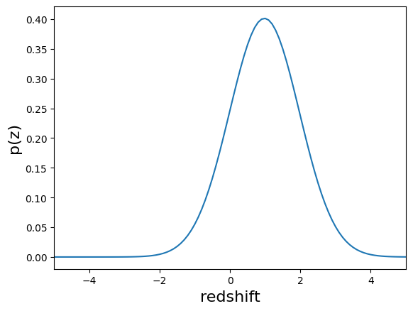
Converting the ensemble
The qp.Ensemble.convert_to function lets you convert ensembles to other representations. To do this you have to provide the original ensemble, the class you want to convert to, and any some keyword arguments to specify details about how to convert to the new class, here are some examples.
bins = np.linspace(-5, 5, 11)
quants = np.linspace(0.01, 0.99, 7)
print("Making hist")
ens_h = ens_n.convert_to(qp.hist_gen, bins=bins)
print("Making interp")
ens_i = ens_n.convert_to(qp.interp_gen, xvals=bins)
print("Making spline")
ens_s = ens_n.convert_to(qp.spline_gen, xvals=bins, method="xy")
#print("Making spline from samples")
#ens_s = ens_n.convert_to(qp.spline_gen, xvals=bins, samples=1000, method="samples")
print("Making quants")
ens_q = ens_n.convert_to(qp.quant_gen, quants=quants)
print("Making mixmod")
ens_m = ens_n.convert_to(qp.mixmod_gen, samples=1000, ncomps=3)
#print("Making flexcode")
#ens_f = ens_n.convert_to(qp.flex_gen, grid=bins, basis_system='cosine')
Making hist
Making interp
Making spline
Making quants
Making mixmod
The qp.convert function also works the more or less the same way, but with slightly different syntax, where you can use the name of the class instead of the class object.
print("Making hist")
ens_h2 = qp.convert(ens_n, "hist", bins=bins)
print("Making interp")
ens_i2 = qp.convert(ens_n, "interp", xvals=bins)
print("Making spline")
ens_s2 = qp.convert(ens_n, "spline", xvals=bins, method="xy")
print("Making quants")
ens_q2 = qp.convert(ens_n, "quant", quants=quants)
print("Making mixmod")
ens_m2 = qp.convert(ens_n, "mixmod", samples=1000, ncomps=3)
Making hist
Making interp
Making spline
Making quants
Making mixmod
Comparing Parametrizations
qp supports quantitative comparisons between different distributions, across parametrizations.
Qualitative Comparisons: Plotting
Let’s visualize the PDF object in order to original and the other representaions. The solid, black line shows the true PDF evaluated between the bounds. The green rugplot shows the locations of the 1000 samples we took. The vertical, dotted, blue lines show the percentiles we asked for, and the hotizontal, dotted, red lines show the 10 equally spaced bins we asked for. Note that the quantiles refer to the probability distribution between the bounds, because we are not able to integrate numerically over an infinite range. Interpolations of each parametrization are given as dashed lines in their corresponding colors. Note that the interpolations of the quantile and histogram parametrizations are so close to each other that the difference is almost imperceptible!
fig, axes = qp.plotting.plot_native(ens_n[15], xlim=(-5.,5.))
qp.plotting.plot_native(ens_h[15], axes=axes)
qp.plotting.plot_native(ens_q[15], axes=axes, label='quantile')
qp.plotting.plot_native(ens_i[15], axes=axes, label='interp')
# qp.plotting.plot_native(ens_s[15], axes=axes, label='spline')
qp.plotting.plot_native(ens_m[15], axes=axes, label='mixmod')
#qp.qp_plot_native(ens_f[15], axes=axes, label='flex')
leg = fig.legend()
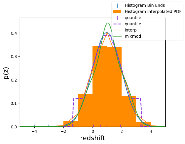
We can also interpolate the function onto an evenly spaced grid point and cache those values with the gridded function.
grid = np.linspace(-3., 3., 100)
gridded = ens_n.pdf(grid)
cached_gridded = ens_n.gridded(grid)[1]
check = gridded - cached_gridded
print(check.min(), check.max())
0.0 0.0
Quantitative Comparisons
symm_lims = np.array([-1., 1.])
all_lims = [symm_lims, 2.*symm_lims, 3.*symm_lims]
Next, let’s compare the different parametrizations to the truth using the Kullback-Leibler Divergence (KLD). The KLD is a measure of how close two probability distributions are to one another – a smaller value indicates closer agreement. It is measured in units of bits of information, the information lost in going from the second distribution to the first distribution. The KLD calculator here takes in a shared grid upon which to evaluate the true distribution and the interpolated approximation of that distribution and returns the KLD of the approximation relative to the truth, which is not in general the same as the KLD of the truth relative to the approximation. Below, we’ll calculate the KLD of the approximation relative to the truth over different ranges, showing that it increases as it includes areas where the true distribution and interpolated distributions diverge.
# for a single pair of pdfs. (the 15th in each ensemble)
klds = qp.metrics.calculate_kld(ens_n, ens_s, limits=symm_lims)
print(klds)
[9.94452805e-04 9.34242455e-04 1.16108771e-03 2.54077451e-03
 3.29974557e-03 4.30372440e-03 1.77895920e-03 1.31020018e-03
 3.54906286e-03 2.29740498e-03 2.78477650e-03 2.90869769e-03
 1.37374792e-03 3.86467531e-03 1.00029562e-03 3.04506068e-04
 3.25792362e-03 4.43438144e-03 3.19806636e-04 3.78991470e-03
 1.76423360e-04 2.58839171e-03 3.51337130e-03 8.26096139e-05
 3.57531619e-03 3.06492530e-03 2.97540295e-03 3.33495641e-03
 3.54809621e-03 4.40593925e-03 3.29327673e-03 3.46441538e-03
 1.74760469e-03 3.28440792e-03 3.48639982e-03 3.52494594e-03
 2.57752631e-03 2.85986774e-03 2.00394486e-03 3.02539298e-03
 1.57123132e-03 1.61732887e-03 3.71373245e-03 3.32434776e-03
 7.47307283e-04 1.39903298e-03 3.86419548e-03 1.80550151e-03
 3.23776210e-03 3.75738584e-03 3.14355281e-03 3.92223709e-03
 3.29191400e-03 2.74557936e-03 2.14416212e-03 3.52685942e-03
 3.35535675e-04 2.66976183e-03 2.34999172e-03 3.75681024e-03
 3.39007362e-03 2.96794341e-03 3.30815597e-03 3.27409606e-03
 4.53316886e-03 3.21754171e-03 3.64618588e-03 1.34644346e-03
 1.42214359e-03 1.91587428e-03 2.09424880e-03 1.94381376e-03
 2.78069573e-03 3.20461047e-03 3.59869714e-03 3.79566519e-03
 4.23593456e-03 3.75274899e-03 1.46803075e-03 4.01393586e-03
 3.80729319e-03 3.57103968e-03 3.10204739e-03 2.90794597e-03
 1.88388500e-03 3.66992289e-03 2.33846661e-03 3.85884373e-03
 1.64200530e-03 2.74925245e-03 2.86163109e-03 2.84125496e-03
 2.79097854e-03 3.24742753e-03 1.96989619e-03 3.27386414e-03
 1.80328139e-03 3.04636065e-03 4.30339038e-03 1.48793407e-03]
# Loop over all the other ensemble types
ensembles = [ens_n, ens_h, ens_i, ens_s, ens_q, ens_m]
for ensemble in ensembles[1:]:
    D = []
    for lims in all_lims:
        klds = qp.metrics.calculate_kld(ens_n, ensemble, limits=lims)
        D.append("%.2e +- %.2e" % (klds.mean(), klds.std()))
    print(ensemble.gen_class.name + ' approximation: KLD over 1, 2, 3, sigma ranges = ' + str(D))
hist approximation: KLD over 1, 2, 3, sigma ranges = ['1.16e-02 +- 3.41e-03', '2.77e-02 +- 4.62e-03', '3.73e-02 +- 4.71e-03']
interp approximation: KLD over 1, 2, 3, sigma ranges = ['3.18e-02 +- 9.99e-03', '2.33e-02 +- 2.52e-03', '1.00e-02 +- 1.80e-03']
broken KLD: (array([ 4.68450416e-03,  4.19474446e-03,  3.02053449e-03,  7.71982562e-04,
       -3.04129678e-04, -2.63188330e-03,  4.17449643e-03,  2.95813071e-03,
       -8.26036400e-04,  1.04752660e-03,  1.74455217e-03,  1.27858247e-03,
        2.90946295e-03, -1.51401320e-03,  2.83585763e-03,  4.15209547e-03,
       -2.22539684e-04, -3.07517483e-03,  3.60610005e-03, -9.18820820e-04,
        3.29306492e-03,  2.60706388e-03, -7.10307631e-04,  2.63429086e-03,
       -8.81630678e-04,  4.16882298e-04,  3.62025553e-04,  4.50733713e-04,
       -6.67240684e-04, -2.98040345e-03, -2.94806123e-04, -6.11958050e-04,
        3.60609623e-03, -3.55619237e-04, -3.11313280e-04,  3.89745401e-05,
        7.76881126e-04,  4.88815735e-04,  2.91835772e-03,  1.10711056e-04,
        2.92819626e-03,  1.56642687e-03, -1.15073511e-03, -4.32230905e-04,
        3.24352756e-03,  3.17078472e-03, -1.20834846e-03,  2.98736900e-03,
       -2.93939080e-04, -1.25164356e-03, -1.15529561e-04, -9.36978884e-04,
        9.84102487e-04,  4.70844889e-04,  3.39901734e-03, -7.49226582e-04,
        2.54767280e-03,  6.06698116e-04,  1.14772877e-03, -1.28030109e-03,
       -4.90264041e-04,  1.72895825e-04, -9.94153474e-05, -1.54418291e-04,
       -3.37297034e-03, -1.25070989e-04, -1.02805245e-03,  3.19266034e-03,
        2.50570124e-03,  3.35222018e-03,  1.46538586e-03,  3.50030584e-03,
        4.88764857e-04,  2.72855845e-04, -6.14890220e-04, -8.39464182e-04,
       -2.50665280e-03, -1.17568182e-03,  4.27975845e-03, -1.86424788e-03,
       -1.39958290e-03, -8.86472811e-04,  7.89840656e-04,  2.26199562e-04,
        1.96223701e-03, -3.34506505e-04,  9.81443639e-04, -1.48266843e-03,
        4.35992148e-03,  5.52527038e-04,  8.19684383e-04,  1.05480910e-03,
        1.24642624e-03,  2.35596505e-04,  1.92416162e-03, -3.36180597e-04,
        3.29414180e-03,  1.33615460e-03, -2.42907326e-03,  3.71332028e-03]), array([[0.21480709, 0.21749946, 0.22020037, ..., 0.00373708, 0.00361584,
        0.00349813],
       [0.2161323 , 0.21869839, 0.22127101, ..., 0.00474778, 0.00460219,
        0.00446057],
       [0.00779041, 0.00800866, 0.00823223, ..., 0.20932189, 0.20700105,
        0.20468593],
       ...,
       [0.14158931, 0.14391833, 0.14626818, ..., 0.00768846, 0.00745295,
        0.00722379],
       [0.07150835, 0.07300708, 0.0745283 , ..., 0.02199224, 0.02141063,
        0.0208419 ],
       [0.19706275, 0.19962204, 0.20219209, ..., 0.00531465, 0.00515131,
        0.00499243]], shape=(100, 400)), array([[0.21418101, 0.21676313, 0.21935903, ..., 0.00363112, 0.00355893,
        0.00348794],
       [0.21555361, 0.21801463, 0.22048675, ..., 0.00466131, 0.004554  ,
        0.00444863],
       [0.00777394, 0.00797602, 0.00818198, ..., 0.20875137, 0.20649745,
        0.20425324],
       ...,
       [0.1413684 , 0.14378629, 0.14623313, ..., 0.00760579, 0.00740721,
        0.00721252],
       [0.07150668, 0.07320197, 0.0749264 , ..., 0.02212104, 0.02147467,
        0.02084142],
       [0.19656473, 0.19906053, 0.20157276, ..., 0.0052233 , 0.00510042,
        0.00497981]], shape=(100, 400)), np.float64(0.010025062656641603))
spline approximation: KLD over 1, 2, 3, sigma ranges = ['2.73e-03 +- 1.07e-03', '2.22e-16 +- 0.00e+00', '1.06e-03 +- 2.66e-04']
broken KLD: (array([-0.01515181, -0.01264715, -0.006195  ,  0.004653  ,  0.00746563,
        0.00782459, -0.01401765, -0.00574039,  0.00929554,  0.00327511,
       -0.00372523, -0.00139672, -0.00547356,  0.00912679, -0.00559099,
       -0.01440558,  0.00720173,  0.00812111, -0.01196785,  0.0037811 ,
       -0.0114534 , -0.00852816,  0.00797938, -0.00927728,  0.00941185,
        0.0028461 ,  0.00449778,  0.00029192,  0.00609035,  0.00812297,
        0.00749223,  0.00785151, -0.01033216,  0.00965906,  0.00353293,
        0.00098453,  0.00428727,  0.00458384, -0.00694476,  0.00728033,
       -0.00571975,  0.00032446,  0.00868386,  0.0102615 , -0.00835141,
       -0.00689684,  0.00481066, -0.0066115 ,  0.01054238,  0.00878969,
        0.00879797,  0.00235819, -0.00293404,  0.00647125, -0.01100582,
        0.00828902, -0.00720452,  0.00545769,  0.00224028,  0.00977512,
        0.0081608 ,  0.00750024,  0.00436939,  0.00569285,  0.00765933,
        0.00659311,  0.00940662, -0.00699885, -0.00345744, -0.00943561,
        0.0008175 , -0.01055442,  0.00565715,  0.00246171,  0.0044022 ,
        0.00316807,  0.00898736,  0.00737635, -0.01351036,  0.00854751,
        0.00987842,  0.01002879,  0.00019544,  0.0079137 , -0.0011912 ,
        0.00165167,  0.00371837,  0.00867126, -0.01456117,  0.00520515,
        0.00164849,  0.0004037 , -0.00033406,  0.00227983, -0.0010981 ,
        0.00955216, -0.00855811, -0.00308198,  0.00590364, -0.01017391]), array([[0.42349542, 0.42393696, 0.42433016, ..., 0.05643776, 0.05523078,
        0.0540434 ],
       [0.41174314, 0.4121608 , 0.41253402, ..., 0.06162162, 0.06037693,
        0.05915095],
       [0.07579057, 0.07716189, 0.07855031, ..., 0.38962363, 0.38907518,
        0.38848937],
       ...,
       [0.40022084, 0.40198969, 0.40371787, ..., 0.09395779, 0.0921671 ,
        0.09039968],
       [0.31388189, 0.316662  , 0.31942828, ..., 0.17460022, 0.17201915,
        0.16945585],
       [0.41294011, 0.41369335, 0.41440167, ..., 0.06844133, 0.06707395,
        0.06572655]], shape=(100, 200)), array([[0.41344567, 0.41344567, 0.41344567, ..., 0.12582315, 0.12582315,
        0.12582315],
       [0.40196895, 0.40196895, 0.40196895, ..., 0.12233046, 0.12233046,
        0.12233046],
       [0.11624193, 0.11624193, 0.11624193, ..., 0.38196249, 0.38196249,
        0.38196249],
       ...,
       [0.38904046, 0.3908945 , 0.39274854, ..., 0.12854826, 0.12854826,
        0.12854826],
       [0.3143948 , 0.31686573, 0.31933666, ..., 0.19215358, 0.18968265,
        0.18721172],
       [0.4074112 , 0.4074112 , 0.4074112 , ..., 0.12398668, 0.12398668,
        0.12398668]], shape=(100, 200)), np.float64(0.010050251256281407))
broken KLD: (array([ 0.2281397 ,  0.21463199,  0.17607167, -0.02818043, -0.02838634,
       -0.04200503,  0.22919222,  0.17227401, -0.02588647, -0.02901532,
        0.18805315,  0.16253383,  0.1757997 , -0.03115452,  0.16893564,
        0.2151364 , -0.02878736, -0.04450566,  0.20038182,  0.09096575,
        0.19936794,  0.21075995, -0.02910036,  0.17866579, -0.02592399,
        0.0676334 , -0.01737656,  0.15553914, -0.03437593, -0.04381869,
       -0.02825073, -0.02890367,  0.217531  , -0.02142171,  0.07174029,
        0.15588357, -0.02943414, -0.03157542,  0.19699455, -0.02646198,
        0.18237673,  0.02426328, -0.02987047, -0.01992505,  0.19106087,
        0.1883204 ,  0.0568071 ,  0.19212014, -0.01786228, -0.03026183,
       -0.02283798,  0.1341371 ,  0.1909409 , -0.02581211,  0.22295864,
       -0.02841578,  0.16545239, -0.02756539,  0.01105602, -0.02772648,
       -0.02722169, -0.02530109,  0.02338856, -0.03288611, -0.04761605,
       -0.03009333, -0.02696975,  0.18782068,  0.15216065,  0.21304685,
        0.04778979,  0.2179855 , -0.02821311,  0.08742275,  0.04914908,
        0.11088334, -0.03853512, -0.03362618,  0.2269938 , -0.03505454,
       -0.02831401, -0.02409141,  0.14916527, -0.02354828,  0.11209779,
        0.14295068, -0.02836341, -0.03214407,  0.23101905, -0.02899158,
        0.08653581,  0.12967196,  0.14429176,  0.09807432,  0.11863317,
       -0.02165133,  0.20608592,  0.18979119,  0.02638907,  0.20880212]), array([[0.21480709, 0.21749946, 0.22020037, ..., 0.00373708, 0.00361584,
        0.00349813],
       [0.2161323 , 0.21869839, 0.22127101, ..., 0.00474778, 0.00460219,
        0.00446057],
       [0.00779041, 0.00800866, 0.00823223, ..., 0.20932189, 0.20700105,
        0.20468593],
       ...,
       [0.14158931, 0.14391833, 0.14626818, ..., 0.00768846, 0.00745295,
        0.00722379],
       [0.07150835, 0.07300708, 0.0745283 , ..., 0.02199224, 0.02141063,
        0.0208419 ],
       [0.19706275, 0.19962204, 0.20219209, ..., 0.00531465, 0.00515131,
        0.00499243]], shape=(100, 400)), array([[0.22799517, 0.23035064, 0.23270612, ..., 0.        , 0.        ,
        0.        ],
       [0.22802472, 0.23025124, 0.23247776, ..., 0.        , 0.        ,
        0.        ],
       [0.        , 0.        , 0.        , ..., 0.22009743, 0.21808702,
        0.21607662],
       ...,
       [0.15903185, 0.16149046, 0.16394907, ..., 0.        , 0.        ,
        0.        ],
       [0.12870825, 0.12870825, 0.12870825, ..., 0.        , 0.        ,
        0.        ],
       [0.21173171, 0.21401894, 0.21630616, ..., 0.        , 0.        ,
        0.        ]], shape=(100, 400)), np.float64(0.010025062656641603))
quant approximation: KLD over 1, 2, 3, sigma ranges = ['2.22e-16 +- 0.00e+00', '2.22e-16 +- 0.00e+00', '3.13e-01 +- 8.10e-02']
broken KLD: (array([ 0.02739331, -0.02497928,  0.01808318,  0.00414511, -0.01021121,
        0.00579893,  0.00911789,  0.00588491, -0.00282479, -0.02427007,
        0.01146296,  0.00504719, -0.00155808,  0.01721526, -0.01491038,
        0.02521797, -0.01928302,  0.00641743,  0.00183972,  0.01104397,
       -0.01562133,  0.00278471,  0.03416723,  0.00280235,  0.00905036,
       -0.00134347,  0.01115165, -0.01200603,  0.01914862, -0.0091121 ,
        0.00406522,  0.0123399 , -0.00554253,  0.01280499, -0.00728399,
       -0.00324863,  0.00855904,  0.00933847,  0.00513032,  0.01792147,
        0.01155602,  0.0042632 , -0.00269884,  0.00335929, -0.00970357,
       -0.00468286,  0.00562772,  0.00270969,  0.02424542,  0.00078183,
       -0.01123928,  0.02417321,  0.01412742,  0.0045499 , -0.02177971,
        0.00213479, -0.00865208, -0.00822742,  0.01056188,  0.01292734,
        0.01245708,  0.00520358, -0.00767716, -0.00813296,  0.02016805,
       -0.01649287,  0.02838408, -0.00645026, -0.00266304, -0.01480981,
       -0.00243719,  0.00938478, -0.00407645, -0.00437454, -0.00235813,
        0.00427361,  0.00676858,  0.02660105, -0.00995084, -0.00016097,
        0.01642087, -0.00247096,  0.01379509,  0.02345884,  0.00608026,
        0.00055131,  0.00468518, -0.01817302,  0.00476744,  0.0046089 ,
        0.01015112,  0.01061943,  0.01010449,  0.01869171,  0.01766595,
        0.00060983, -0.00115217,  0.00193384,  0.00939428,  0.00541366]), array([[0.42349542, 0.42393696, 0.42433016, ..., 0.05643776, 0.05523078,
        0.0540434 ],
       [0.41174314, 0.4121608 , 0.41253402, ..., 0.06162162, 0.06037693,
        0.05915095],
       [0.07579057, 0.07716189, 0.07855031, ..., 0.38962363, 0.38907518,
        0.38848937],
       ...,
       [0.40022084, 0.40198969, 0.40371787, ..., 0.09395779, 0.0921671 ,
        0.09039968],
       [0.31388189, 0.316662  , 0.31942828, ..., 0.17460022, 0.17201915,
        0.16945585],
       [0.41294011, 0.41369335, 0.41440167, ..., 0.06844133, 0.06707395,
        0.06572655]], shape=(100, 200)), array([[0.446855  , 0.44608073, 0.44521216, ..., 0.05417553, 0.05271037,
        0.05127141],
       [0.41417853, 0.41630419, 0.41836466, ..., 0.06807568, 0.06659231,
        0.0651268 ],
       [0.09101994, 0.09248213, 0.09395102, ..., 0.39135641, 0.39063209,
        0.38985117],
       ...,
       [0.40048357, 0.40290879, 0.4052838 , ..., 0.1016475 , 0.09976193,
        0.09789271],
       [0.30539743, 0.30846356, 0.31153756, ..., 0.16669128, 0.16479411,
        0.16290872],
       [0.48464017, 0.48582725, 0.48686855, ..., 0.06812436, 0.06633472,
        0.06457083]], shape=(100, 200)), np.float64(0.010050251256281407))
broken KLD: (array([ 0.01384091,  0.00419831,  0.01650453, -0.00370236,  0.00205226,
        0.00213691,  0.00817146,  0.01593005,  0.00747121, -0.00428089,
        0.00544181,  0.01519281,  0.01200896,  0.00186904,  0.00040221,
        0.02305078, -0.00247257,  0.00442871,  0.02213348,  0.01238356,
        0.01370472,  0.00699574,  0.01866207, -0.00607494, -0.00017773,
        0.008718  ,  0.00804134,  0.00742565,  0.01868142,  0.00538828,
        0.00648072, -0.00226095,  0.00892763,  0.00135899,  0.00176784,
        0.00513052, -0.00213506,  0.00796628,  0.0171669 ,  0.01382264,
       -0.0025338 , -0.00787119,  0.00136137,  0.00014555,  0.01719793,
        0.0119689 ,  0.00702498,  0.00330315,  0.00982877, -0.00570979,
        0.00017255,  0.00417561,  0.016538  , -0.00338504,  0.01391101,
       -0.0016523 , -0.00709867,  0.0051461 ,  0.00895195,  0.01521222,
       -0.00307481,  0.00507619,  0.00418878,  0.00785625,  0.00438256,
        0.00715289,  0.00855202,  0.00427982,  0.01402843, -0.00193352,
        0.01399987,  0.01411857,  0.00591221,  0.00608147,  0.00131097,
        0.01645596, -0.00737442,  0.00622728,  0.00770584, -0.0075742 ,
       -0.00419611, -0.00025852,  0.0065429 ,  0.013215  ,  0.02731975,
       -0.003361  ,  0.00894015, -0.00292027,  0.01012616, -0.00078114,
       -0.00305679,  0.00265698,  0.01373126,  0.01513908,  0.00715418,
        0.0008051 ,  0.00487668,  0.01211   ,  0.00456265,  0.00611474]), array([[0.21480709, 0.21749946, 0.22020037, ..., 0.00373708, 0.00361584,
        0.00349813],
       [0.2161323 , 0.21869839, 0.22127101, ..., 0.00474778, 0.00460219,
        0.00446057],
       [0.00779041, 0.00800866, 0.00823223, ..., 0.20932189, 0.20700105,
        0.20468593],
       ...,
       [0.14158931, 0.14391833, 0.14626818, ..., 0.00768846, 0.00745295,
        0.00722379],
       [0.07150835, 0.07300708, 0.0745283 , ..., 0.02199224, 0.02141063,
        0.0208419 ],
       [0.19706275, 0.19962204, 0.20219209, ..., 0.00531465, 0.00515131,
        0.00499243]], shape=(100, 400)), array([[0.22403765, 0.22646222, 0.22890685, ..., 0.00097237, 0.00092168,
        0.00087339],
       [0.22840121, 0.2299305 , 0.23142881, ..., 0.0024394 , 0.00233163,
        0.00222809],
       [0.00701421, 0.00726882, 0.00753112, ..., 0.22137916, 0.21966593,
        0.21794967],
       ...,
       [0.14790408, 0.14970217, 0.15150989, ..., 0.00566051, 0.00543911,
        0.00522522],
       [0.07729577, 0.07882766, 0.08037617, ..., 0.02825709, 0.02751517,
        0.02678741],
       [0.19304965, 0.19496647, 0.19689044, ..., 0.00094411, 0.00088947,
        0.00083771]], shape=(100, 400)), np.float64(0.010025062656641603))
broken KLD: (array([ 0.00378958, -0.00378161,  0.00104701, -0.0023948 ,  0.0026196 ,
        0.00391186,  0.00264447,  0.00494666,  0.00325421,  0.0033902 ,
        0.00092017,  0.00916339,  0.00179869,  0.00657494, -0.00631177,
        0.00630323,  0.00264184,  0.00604665,  0.00832261,  0.00388303,
        0.00886239,  0.00149142,  0.00766059,  0.00216347,  0.0035279 ,
        0.00488841,  0.00499961,  0.00533331,  0.00639679,  0.00343953,
        0.00616691,  0.00120871,  0.00130745,  0.00520413,  0.00474218,
        0.00369451, -0.00088986,  0.00551244,  0.00542317,  0.00617076,
       -0.00243746, -0.00456562,  0.0007951 ,  0.00185448,  0.01108645,
        0.00510024,  0.0023223 ,  0.00119577,  0.0018091 ,  0.00353733,
        0.00117213,  0.00414695,  0.00630714,  0.00069593,  0.00457642,
        0.00080914,  0.00786227,  0.00197201,  0.00113417,  0.00436316,
        0.00132715,  0.00190744,  0.00571767,  0.00405837,  0.0048351 ,
        0.00474929,  0.00402731, -0.00047956,  0.01036818,  0.00083253,
        0.00686828,  0.00419137,  0.00250311,  0.00495151,  0.00166273,
        0.0066886 ,  0.00430553,  0.00589287, -0.00021817,  0.00522368,
        0.00281805,  0.00111103,  0.00209327,  0.00355702,  0.01084492,
        0.00100051,  0.00431212,  0.00174467,  0.00814431, -0.00145734,
        0.00319311,  0.00115533,  0.00507632,  0.00381639,  0.00536309,
        0.00036218,  0.00185139,  0.00289716,  0.00167501,  0.00634611]), array([[3.48882925e-02, 3.57304712e-02, 3.65887986e-02, ...,
        7.92395259e-05, 7.58012688e-05, 7.25039153e-05],
       [3.86652056e-02, 3.95480166e-02, 4.04466155e-02, ...,
        1.24672238e-04, 1.19556052e-04, 1.14637437e-04],
       [3.02962942e-04, 3.14490609e-04, 3.26425066e-04, ...,
        4.25457766e-02, 4.16667978e-02, 4.08019991e-02],
       ...,
       [1.52593992e-02, 1.56959659e-02, 1.61430973e-02, ...,
        1.91660535e-04, 1.83595387e-04, 1.75848650e-04],
       [4.94809121e-03, 5.11236858e-03, 5.28146849e-03, ...,
        8.41373378e-04, 8.09421365e-04, 7.78589669e-04],
       [3.11232464e-02, 3.18782572e-02, 3.26479612e-02, ...,
        1.36586259e-04, 1.30933485e-04, 1.25500733e-04]], shape=(100, 600)), array([[3.71479765e-02, 3.82607230e-02, 3.93957641e-02, ...,
        1.27530326e-06, 1.17759059e-06, 1.08707912e-06],
       [2.85490831e-02, 2.96204013e-02, 3.07215344e-02, ...,
        8.42786494e-06, 7.86883206e-06, 7.34515253e-06],
       [7.16442134e-05, 7.57712951e-05, 8.01197548e-05, ...,
        4.79003658e-02, 4.66856388e-02, 4.54911255e-02],
       ...,
       [1.98298074e-02, 2.04412468e-02, 2.10666946e-02, ...,
        3.55568850e-05, 3.34215377e-05, 3.14074807e-05],
       [4.11232803e-03, 4.27811277e-03, 4.44964824e-03, ...,
        7.35399848e-04, 7.01788711e-04, 6.69577522e-04],
       [2.72910269e-02, 2.81837695e-02, 2.90976970e-02, ...,
        4.80542054e-07, 4.38008265e-07, 3.99106847e-07]], shape=(100, 600)), np.float64(0.01001669449081803))
mixmod approximation: KLD over 1, 2, 3, sigma ranges = ['2.22e-16 +- 0.00e+00', '2.22e-16 +- 0.00e+00', '2.22e-16 +- 0.00e+00']
The progression of KLD values should follow that of the root mean square error (RMSE), another measure of how close two functions are to one another. The RMSE also increases as it includes areas where the true distribution and interpolated distribution diverge. Unlike the KLD, the RMSE is symmetric, meaning the distance measured is not that of one distribution from the other but of the symmetric distance between them.
for ensemble in ensembles[1:]:
    D = []
    for lims in all_lims:
        rmses = qp.metrics.calculate_rmse(ens_n, ensemble, limits=lims)
        D.append("%.2e +- %.2e" % (rmses.mean(), rmses.std()))
    print(ensemble.gen_class.name + ' approximation: RMSE over 1, 2, 3, sigma ranges = ' + str(D))
---------------------------------------------------------------------------
ValueError                                Traceback (most recent call last)
Cell In[35], line 4
      2 D = []
      3 for lims in all_lims:
----> 4     rmses = qp.metrics.calculate_rmse(ens_n, ensemble, limits=lims)
      5     D.append("%.2e +- %.2e" % (rmses.mean(), rmses.std()))
      6 print(ensemble.gen_class.name + ' approximation: RMSE over 1, 2, 3, sigma ranges = ' + str(D))

File ~/checkouts/readthedocs.org/user_builds/qp/envs/latest/lib/python3.10/site-packages/qp/metrics/metrics.py:236, in calculate_rmse(p, q, limits, dx)
    210 """
    211 Calculates the Root Mean Square Error between two qp.Ensemble objects.
    212
   (...)
    233 TO DO: change dx to N
    234 """
    235 if p.shape != q.shape:
--> 236     raise ValueError(
    237         "Cannot calculate RMSE between two ensembles with different shapes"
    238     )
    240 # Make a grid from the limits and resolution
    241 grid = _calculate_grid_parameters(limits, dx)

ValueError: Cannot calculate RMSE between two ensembles with different shapes
Both the KLD and RMSE metrics suggest that the quantile approximation is better in the high density region, but samples work better when the tails are included. We might expect the answer to the question of which approximation to use to depend on the application, and whether the tails need to be captured or not.
Storing and retreiving ensembles
You can store and retrieve ensembles from disk using the qp.Ensemble.write_to and qp.read methods.
These work in two steps, first they convert the Ensemble data to astropy.table objects, and then they write the tables. This means you can store the data in any format support by astropy.
tabs = ens_n.build_tables()
print(tabs.keys())
print()
print("Meta Data")
print(tabs['meta'])
print()
print("Object Data")
print(tabs['data'])
dict_keys(['meta', 'data'])

Meta Data
{'pdf_name': array([b'norm'], dtype='|S4'), 'pdf_version': array([0])}

Object Data
{'loc': array([[-0.90392493],
       [-0.90125972],
       [ 0.84072264],
       [-0.47245378],
       [ 0.30410875],
       [ 0.14738051],
       [ 0.82518467],
       [-0.81991849],
       [ 0.16271236],
       [-0.53346303],
       [ 0.65450034],
       [-0.61180125],
       [-0.81035422],
       [ 0.12704387],
       [ 0.85499231],
       [ 0.98128315],
       [-0.32078515],
       [-0.07821505],
       [ 0.97318855],
       [ 0.4036157 ],
       [-0.99130883],
       [-0.71884708],
       [ 0.25440321],
       [ 0.99755856],
       [-0.14874853],
       [-0.48977765],
       [ 0.44540444],
       [-0.54752602],
       [-0.33970735],
       [ 0.08990351],
       [ 0.30345041],
       [ 0.26679232],
       [-0.80611437],
       [-0.16529811],
       [-0.43713719],
       [-0.51701087],
       [ 0.48151596],
       [-0.45125759],
       [ 0.75630993],
       [-0.33838388],
       [-0.79031407],
       [-0.67649716],
       [-0.18674876],
       [-0.08728444],
       [ 0.90382912],
       [-0.81901869],
       [-0.35776221],
       [ 0.77313886],
       [ 0.04095407],
       [-0.17314325],
       [-0.24607757],
       [-0.44406692],
       [ 0.60563549],
       [ 0.39365009],
       [ 0.77461542],
       [-0.23532555],
       [ 0.95133402],
       [ 0.4362138 ],
       [-0.55976062],
       [ 0.06894475],
       [-0.25799105],
       [-0.33333262],
       [ 0.42383144],
       [ 0.38071306],
       [ 0.09219983],
       [ 0.35076821],
       [-0.13834841],
       [ 0.82560588],
       [-0.78361045],
       [ 0.78395461],
       [-0.6201394 ],
       [-0.78914025],
       [ 0.42104143],
       [-0.49143627],
       [ 0.39849645],
       [ 0.42492522],
       [ 0.00129182],
       [-0.25840744],
       [ 0.85069367],
       [-0.14982995],
       [ 0.00488018],
       [-0.07396283],
       [ 0.56578949],
       [-0.31875677],
       [-0.69453642],
       [ 0.48618903],
       [-0.51694171],
       [-0.16656967],
       [-0.84005997],
       [ 0.43896394],
       [-0.53930595],
       [-0.57719774],
       [-0.60032567],
       [ 0.494023  ],
       [ 0.68437362],
       [-0.17609331],
       [-0.78855249],
       [-0.62582628],
       [-0.25865192],
       [-0.83099183]]), 'scale': array([[0.93708462],
       [0.96383958],
       [1.01432364],
       [1.0740079 ],
       [1.03297081],
       [0.93385047],
       [0.90379927],
       [1.0085031 ],
       [1.03113432],
       [1.07896496],
       [0.92861533],
       [0.94205616],
       [1.00710169],
       [0.994723  ],
       [1.0348385 ],
       [0.99390875],
       [1.03355292],
       [0.92176644],
       [1.018909  ],
       [0.93812368],
       [1.03789841],
       [0.90366831],
       [1.01800903],
       [1.07411633],
       [1.02971648],
       [0.9916151 ],
       [1.0248521 ],
       [0.92879133],
       [0.98962311],
       [0.92510611],
       [1.03401687],
       [1.02137726],
       [0.93480698],
       [1.06536527],
       [0.96166302],
       [0.92259413],
       [1.0642168 ],
       [1.03821053],
       [0.94975255],
       [1.05922085],
       [0.99044194],
       [1.09731471],
       [1.00579871],
       [1.06908865],
       [1.02262127],
       [0.98896855],
       [0.94443622],
       [0.96547427],
       [1.08308258],
       [1.00237389],
       [1.06870771],
       [0.909681  ],
       [0.90323163],
       [1.07839419],
       [0.90872419],
       [1.02061757],
       [1.0754396 ],
       [1.07182866],
       [1.05539158],
       [1.01404228],
       [1.03329547],
       [1.0686511 ],
       [0.98973511],
       [1.01113603],
       [0.90612842],
       [1.02926358],
       [1.02185694],
       [0.99151396],
       [1.0308947 ],
       [0.933155  ],
       [1.05627655],
       [0.92247447],
       [1.06252327],
       [0.9725469 ],
       [0.96289498],
       [0.92995226],
       [0.95241795],
       [0.98599823],
       [0.92349023],
       [0.9722631 ],
       [1.00961124],
       [1.03791645],
       [0.9460872 ],
       [1.08133308],
       [1.03265878],
       [0.9203088 ],
       [1.08172987],
       [0.99017395],
       [0.90624243],
       [1.05930152],
       [0.99258993],
       [0.97270617],
       [0.96469354],
       [0.96585756],
       [1.02642564],
       [1.06506615],
       [0.9471749 ],
       [0.91721924],
       [0.91607908],
       [0.9509645 ]])}
Here is a loopback test showing that we get the same results before and after a write/read cycle.
suffix_list = ['_n', '_h', '_i', '_s', '_q', '_m']
filetypes = ['fits', 'hf5']
for ens, suffix in zip(ensembles, suffix_list):
    for ft in filetypes:

        outfile = "test%s.%s" % (suffix, ft)
        metafile = "test%s_meta.%s" % (suffix, ft)

        pdf_1 = ens.pdf(bins)
        ens.write_to(outfile)
        ens_r = qp.read(outfile)
        pdf_2 = ens_r.pdf(bins)

        check = pdf_1 - pdf_2
        print(suffix, ft, check.min(), check.max())

        os.unlink(outfile)
        try:
            os.unlink(metafile)
        except Exception:
            pass
_n fits 0.0 0.0
_n hf5 0.0 0.0
_h fits -1.1102230246251565e-16 5.551115123125783e-17
_h hf5 -1.1102230246251565e-16 5.551115123125783e-17
_i fits -1.1102230246251565e-16 5.551115123125783e-17
_i hf5 -1.1102230246251565e-16 5.551115123125783e-17
_s fits 0.0 0.0
_s hf5 0.0 0.0
_q fits 0.0 0.0
_q hf5 0.0 0.0
_m fits 0.0 0.0
_m hf5 0.0 0.0
Finally, we can compare the moments of each approximation and compare those to the moments of the true distribution.
which_moments = range(3)
all_moments = []
for ens in ensembles:
    moments = []
    for n in which_moments:
        moms = qp.metrics.calculate_moment(ens, n, limits=(-3, 3))
        moments.append("%.2e +- %.2e" % (moms.mean(), moms.std()))
    all_moments.append(moments)

print('moments: '+str(which_moments))
for ens, mom in zip(ensembles, all_moments):
    print(ens.gen_class.name+': '+str(mom))
moments: range(0, 3)
norm: ['9.92e-01 +- 5.92e-03', '-4.27e-02 +- 5.33e-01', '1.22e+00 +- 2.23e-01']
hist: ['9.93e-01 +- 6.13e-03', '-4.37e-02 +- 5.31e-01', '1.38e+00 +- 2.16e-01']
interp: ['9.88e-01 +- 7.77e-03', '-4.18e-02 +- 5.18e-01', '1.34e+00 +- 1.98e-01']
spline: ['9.91e-01 +- 6.03e-03', '-4.28e-02 +- 5.34e-01', '1.23e+00 +- 2.27e-01']
quant: ['1.07e+00 +- 1.30e-02', '-4.88e-02 +- 5.77e-01', '1.56e+00 +- 2.17e-01']
mixmod: ['9.94e-01 +- 6.57e-03', '-4.41e-02 +- 5.39e-01', '1.25e+00 +- 2.32e-01']